Multilevel Modeling in Biomedical Research: A Complete Guide to Analyzing Hierarchical Data Across the Drug Development Cycle
This comprehensive article provides researchers, scientists, and drug development professionals with an in-depth exploration of multilevel modeling (MLM) applications throughout biomedical research cycles.
Multilevel Modeling in Biomedical Research: A Complete Guide to Analyzing Hierarchical Data Across the Drug Development Cycle
Abstract
This comprehensive article provides researchers, scientists, and drug development professionals with an in-depth exploration of multilevel modeling (MLM) applications throughout biomedical research cycles. Covering foundational concepts to advanced implementation, it demonstrates how MLM addresses hierarchical data structures in everything from single-case experimental designs to large-scale clinical trials. The content explores methodological frameworks within Model-Informed Drug Development (MIDD), offers practical troubleshooting strategies, compares MLM performance against alternative statistical approaches, and provides validation techniques for ensuring robust analytical outcomes in pharmaceutical and clinical research settings.
Understanding Multilevel Modeling: Core Principles for Hierarchical Data in Biomedical Research
What is Multilevel Modeling? Defining Hierarchical Structures in Biomedical Data
Multilevel models (MLMs), also known as hierarchical linear models or mixed-effects models, are a class of statistical techniques designed to analyze data with inherent hierarchical or nested structures [1]. In biomedical research, such data structures are the rule rather than the exception [2]. Patients are naturally nested within physicians, who are nested within clinics, which in turn may be nested within hospitals or geographic regions [3]. Similarly, longitudinal studies feature repeated measurements nested within individual patients [1]. Multilevel modeling provides an appropriate analytical framework for these complex data structures by explicitly modeling variability at each level of the hierarchy [4].
The fundamental insight of multilevel modeling recognizes that observations clustered within the same higher-level unit (e.g., patients treated by the same physician) often share more similarities with each other than with observations from different units [3]. This within-cluster homogeneity violates the standard statistical assumption of independent observations. Multilevel models correct for this non-independence while simultaneously allowing researchers to investigate how factors at different levels of the hierarchy interact to influence outcomes [5]. For example, MLMs can examine how patient-level characteristics (level 1) and physician-level practices (level 2) jointly affect treatment outcomes [3].
The application of multilevel modeling in biomedical research has grown immensely over the past decade [4]. A systematic review of literature from 2010-2020 found that 46.2% of applied multilevel modeling studies were in health/epidemiology, with 78.5% being two-level models [4]. This growth reflects increasing recognition that biomedical phenomena are inherently multilevel, influenced by factors ranging from molecular processes to healthcare system characteristics [4] [2].
Key Concepts and Statistical Foundations
Hierarchical Data Structures
Multilevel models define hierarchical structures through their level organization. The finest scale at which the response variable is measured is called the lower level, while aggregate scales are referred to as higher levels [4]. In a typical biomedical example with patients nested within clinics:
- Level 1: Patients (individual measurements)
- Level 2: Clinics (groups of patients)
More complex hierarchies are possible, such as patients (level 1) within physicians (level 2) within hospitals (level 3) [3]. Longitudinal studies represent another common hierarchical structure where repeated measurements (level 1) are nested within patients (level 2) [1].
The Multilevel Equation System
Multilevel models are characterized by their hierarchical equation system. For a simple two-level model with one level-1 predictor [1]:
Level 1 (Within-group) Equation: Yij = β0j + β1jXij + eij
Level 2 (Between-group) Equations: β0j = γ00 + γ01wj + u0j β1j = γ10 + γ11wj + u1j
Where:
- Yij is the outcome for individual i in group j
- Xij is a level-1 predictor for individual i in group j
- β0j and β1j are the intercept and slope that vary across groups
- γ00 and γ10 are the average intercept and slope across groups
- wj is a level-2 predictor
- γ01 and γ11 are the effects of the level-2 predictor on the intercept and slope
- u0j and u1j are level-2 residuals (random effects)
- eij is the level-1 residual
Types of Multilevel Models
Table 1: Types of Multilevel Models and Their Applications
| Model Type | Key Characteristics | Biomedical Application Example |
|---|---|---|
| Random Intercepts | Intercepts vary across groups; slopes are fixed | Examining baseline blood pressure variation across clinics while assuming the effect of medication dosage is constant |
| Random Slopes | Slopes vary across groups; intercepts are fixed | Modeling how the relationship between exercise duration and weight loss varies across different rehabilitation centers |
| Random Intercepts and Slopes | Both intercepts and slopes vary across groups | Studying how both baseline cholesterol levels and the effect of dietary intervention vary across hospitals |
| Cross-Classified | Units nested in multiple non-hierarchical classifications | Patients nested within both physicians and neighborhoods [2] |
Key Assumptions
Multilevel models operate under several key statistical assumptions [1]:
- Linearity: Relationships between variables are linear (though nonlinear extensions exist)
- Normality: Residuals at each level are normally distributed
- Homoscedasticity: Residuals exhibit constant variance
- Independence: Level-1 and level-2 residuals are uncorrelated
Violations of these assumptions may require transformations, different distributional specifications, or robust standard errors [1].
Applications in Biomedical Research
Table 2: Application of Multilevel Models Across Biomedical Fields (2010-2020) [4]
| Field of Application | Percentage of Articles | Common Model Types | Study Designs |
|---|---|---|---|
| Health/Epidemiology | 46.2% | Two-level (78.5%), Multivariate | Cross-sectional (83.1%) |
| Social Life | 16.9% | Random intercept, Random slope | Longitudinal (9.2%) |
| Education and Psychology | 15.4% | Cross-classified | Repeated measures (6.2%) |
| Other Fields | 21.5% | Mixed effects | Mixed designs |
Specific Biomedical Applications
Multilevel models have been employed across diverse biomedical domains. In epidemiology, they estimate effects between conditions such as smoking, asthma, mental health, and cancer while accounting for geographic clustering [4]. In pharmacology, physiologically based pharmacokinetic/pharmacodynamic (PBPK/PD) modeling uses multilevel frameworks to understand drug response variability across individuals and populations [6].
Physical activity research has effectively utilized multilevel modeling to validate measurement approaches. A 2025 study compared ecological momentary assessment (EMA) with traditional physical activity measures using multilevel modeling to account for repeated measurements nested within participants [7]. The models demonstrated that EMA and the Bouchard Physical Activity Record exhibited better performance in modeling accelerometer data compared to the Global Physical Activity Questionnaire (EMA daily: β=.387, P<.001; BAR daily: β=.394, P<.001; GPAQ: β=.281, P<.001) [7].
In health services research, multilevel models disentangle the heterogeneity in prescribing behaviors among physicians. A Scottish study used mixed effects modeling to explore whether "high-risk-prescribing culture" was driven by individual physicians or practice-level culture, finding that high-risk prescribing was more of an individual-physician issue than a practice-level phenomenon [2].
Experimental Protocols and Implementation
Protocol: Implementing a Two-Level Model for Physical Activity Assessment Validation
Objective: To validate smartphone-delivered Ecological Momentary Assessment (EMA) against accelerometer data and traditional physical activity questionnaires using multilevel modeling.
Materials and Equipment:
- ActiGraph GT3X+ accelerometer
- Smartphones with survey capability
- GPAQ (Global Physical Activity Questionnaire)
- BAR (Bouchard Physical Activity Record) adaptation
Procedure:
- Participant Recruitment: Recruit adult participants (18+) capable of daily physical activity with access to mobile phones [7].
- Baseline Assessment: On day 0, measure body composition and handgrip strength; administer GPAQ.
- Accelerometer Deployment: Instruct participants to wear ActiGraph GT3X+ over the right waist within an anterior axillary line for 7 consecutive days (days 1-6), removing only for water activities.
- EMA Implementation: Deliver physical activity questionnaires via SMS with 2-hour intervals between 8 AM and 10 PM on 1 weekday and 1 weekend day.
- BAR Administration: Participants complete the adapted Bouchard Physical Activity Record daily between days 1-6.
- Data Processing:
- Process accelerometer data using Freedson algorithm for METs estimation
- Apply GPAQ analysis guidelines for data cleaning
- Remove EMA records with less than 6 reports per day
- Multilevel Modeling:
- Specify two-level model with repeated observations (level 1) nested within participants (level 2)
- Include fixed effects for assessment type and covariates
- Include random intercepts for participants
- Estimate using maximum likelihood or Bayesian methods
Statistical Analysis:
- Use multilevel modeling to account for the hierarchical data structure
- Compare parameter estimates (β coefficients) across assessment methods
- Evaluate model fit using information criteria (AIC, BIC)
Protocol: Analyzing Physician Practice Patterns in Prescribing
Objective: To examine the effect of physician advice on patient outcomes while accounting for clustering of patients within physicians and practices.
Materials:
- Electronic health records or survey data
- Statistical software with multilevel modeling capabilities
Procedure:
- Data Structure Setup: Organize data with patients (level 1) nested within physicians (level 2) nested within practices (level 3).
- Variable Definition:
- Level 1 (Patient): Outcome variable (e.g., alcohol-free weeks), patient characteristics, hours of physician advice
- Level 2 (Physician): Physician characteristics, years of experience
- Level 3 (Practice): Practice setting (urban/rural), practice size
- Model Building:
- Start with unconditional model (no predictors) to calculate intraclass correlation
- Add level-1 predictors (e.g., patient characteristics, hours of advice)
- Add level-2 and level-3 predictors
- Consider cross-level interactions (e.g., between practice setting and physician advice)
- Model Estimation: Use restricted maximum likelihood or Bayesian estimation
- Interpretation: Partition variance across levels; interpret fixed effects and variance components
Visualization of Multilevel Structures
Hierarchical Data Structure in Biomedical Research
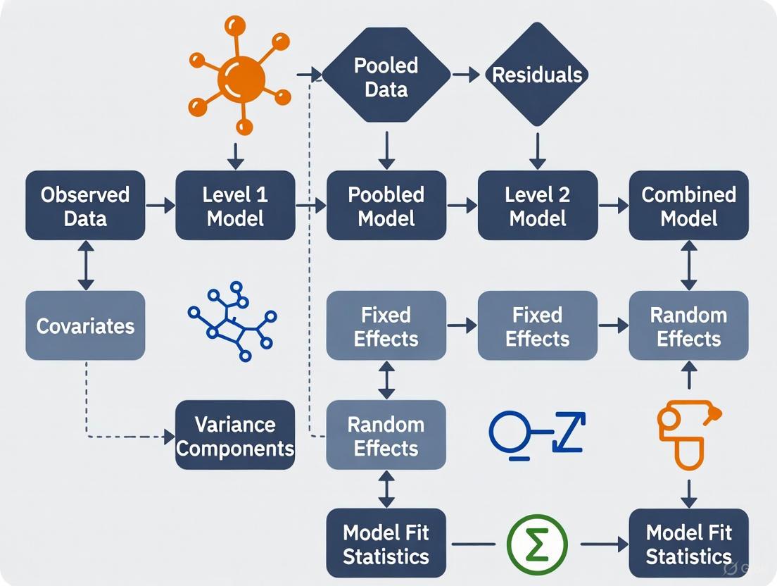
Multilevel Model Estimation Workflow
The Scientist's Toolkit
Research Reagent Solutions for Multilevel Modeling
Table 3: Essential Software Tools for Multilevel Modeling in Biomedical Research
| Software Tool | Primary Function | Key Features for Multilevel Modeling |
|---|---|---|
| R (lme4, nlme) | Statistical computing | Extensive package ecosystem, flexible model specification, open-source |
| Stata (mixed) | Statistical analysis | Straightforward syntax, comprehensive survey weight handling |
| IBM SPSS (MIXED) | Statistical analysis | GUI and syntax options, accessible for beginners |
| Mplus | Structural equation modeling | Advanced multilevel capabilities, latent variable modeling |
| MLwiN | Multilevel modeling | Specialized for multilevel analysis, Bayesian estimation |
| SAS (PROC MIXED) | Statistical analysis | Robust enterprise solution, handling complex covariance structures |
Handling Complex Survey Weights
When working with complex survey data that includes design weights, analysts should scale weights using two primary methods [8]:
- Method A: Scale weights so they sum to the cluster sample size
- Method B: Scale weights so they sum to the effective cluster size
Current recommendations suggest fitting MLMs using both scaled-weighted and unweighted data, with comparisons across methods providing greater confidence in results [8].
Multilevel modeling represents an essential statistical approach for biomedical researchers working with hierarchical data structures. By properly accounting for nested data relationships, these models enable accurate parameter estimation and appropriate inferences that would be compromised using traditional statistical methods. As biomedical research continues to recognize the multifaceted nature of health determinants across biological, clinical, and social levels, multilevel modeling provides the necessary analytical framework to investigate these complex relationships. Future directions include greater integration of spatial effects into multilevel models, improved handling of causal inference in hierarchical data, and continued development of accessible software implementations [4] [2].
Multilevel modeling (MLM), also known as mixed-effects modeling or hierarchical linear modeling, provides a robust statistical framework for analyzing data with nested or clustered structures commonly encountered in scientific research [1] [9]. These models are particularly valuable in drug development and biomedical research where data often exhibit hierarchical organization—such as repeated measurements within patients, patients within clinical sites, or observations within experimental batches. Unlike traditional statistical methods that assume independence of observations, multilevel models explicitly account for the dependency inherent in clustered data, leading to more accurate estimates and inferences [9] [10].
The fundamental components of multilevel models include random intercepts, random slopes, and variance components, which together enable researchers to partition variability across different levels of the data hierarchy [11] [1]. This partitioning allows for more nuanced research questions that extend beyond traditional "fixed effect" analyses, enabling investigators to simultaneously examine relationships between variables and variability across contextual units [11]. For researchers working with cyclical data or longitudinal interventions, these models offer particular advantages in modeling change over time while accounting for individual differences in response patterns [12].
Core Terminology and Definitions
Random Intercepts
Random intercepts capture group-specific deviations from the overall average response, allowing the baseline outcome level to vary across clusters or subjects [11]. In a random intercept model, each group (e.g., school, clinical site, patient) has its own regression line that is parallel to the overall average line but shifted upward or downward based on the group's characteristics [11]. Formally, the random intercept model extends the standard linear model by including a group-specific random effect:
y_ij = β_0 + β_1*x_ij + u_j + e_ij [9]
Where:
y_ijrepresents the outcome for observation i in group jβ_0is the overall intercept (fixed effect)β_1is the slope coefficient for the predictor x (fixed effect)u_jis the random intercept for group j (representing the deviation of group j from the overall intercept)e_ijis the residual error term
As explained in the presentation by Pillinger, "for the random intercept model, the intercept for the overall regression line is still β0 but for each group line the intercept is β0 + uj" [11]. This terminology can sometimes be confusing, as sometimes the entire group-specific intercept (β0 + uj) is referred to as the random intercept, while other times only the deviation uj is called the random intercept [11].
Random Slopes
Random slopes extend this concept by allowing the relationship between predictors and outcomes to vary across groups, recognizing that effects may not be uniform across all clusters [12]. While random intercept models assume parallel regression lines for different groups, random slope models permit these lines to have different slopes, representing differential effects of explanatory variables across groups [12].
The random slope model incorporates an additional random effect for the slope:
y_ij = β_0 + u_0j + (β_1 + u_1j)*x_ij + e_ij [9]
Where:
u_1jis the random slope for group j (representing the deviation of group j's slope from the overall slope β_1)u_0jis the random intercept for group j- Other terms are as defined previously
As Pillinger explains in her presentation on random slope models, "unlike a random intercept model, a random slope model allows each group line to have a different slope and that means that the random slope model allows the explanatory variable to have a different effect for each group" [12]. This flexibility is particularly valuable when researching treatment effects or biological processes that may operate differently across contexts or populations.
Variance Components
Variance components represent the variances of the random terms in a mixed effects model and quantify how much of the total variation in the response can be attributed to each level of the hierarchy [13]. In a basic two-level random intercept model, there are two variance components: the variance of the group-level random intercepts (σ²u) and the variance of the residual errors (σ²e) [11] [13].
These variance components allow researchers to answer questions about the distribution of variability across levels. For example, in a study of patients within hospitals, the variance components would indicate how much variation in outcomes exists between hospitals versus between patients within the same hospital [11]. The intraclass correlation coefficient (ICC), calculated as σ²u / (σ²u + σ²_e), quantifies the proportion of total variance that lies between groups [9].
Table 1: Interpretation of Variance Components in a Mixed Effects Model
| Component | Symbol | Interpretation | Research Question Example |
|---|---|---|---|
| Level 2 Variance | σ²_u | Unexplained variation between groups after controlling for explanatory variables | How much variation in patient outcomes is between clinical sites? |
| Level 1 Variance | σ²_e | Unexplained variation within groups after controlling for explanatory variables | How much variation in patient outcomes remains within each clinical site? |
| Total Variance | σ²u + σ²e | Total unexplained variation in the response variable | What is the overall unexplained variability in the treatment response? |
Analytical Protocols for Multilevel Modeling
Model Specification Workflow
The process of developing multilevel models follows a systematic sequence to ensure appropriate model specification and interpretation [1] [9]. The workflow begins with assessing whether the data structure necessitates multilevel modeling, proceeds through model specification and estimation, and concludes with model diagnostics and interpretation.
Protocol 1: Random Intercept Model Implementation
Purpose: To implement a random intercept model that accounts for group-level variability while estimating the effects of explanatory variables.
Materials and Software Requirements:
- Statistical software capable of fitting mixed effects models (R with lme4 package, SAS PROC MIXED, Stata mixed command, Python statsmodels)
- Dataset with appropriate nested structure
- Computational resources sufficient for maximum likelihood estimation
Procedure:
- Data Preparation: Structure the data in long format with explicit identifiers for grouping variables. Ensure the response variable is examined at the lowest level of analysis [1].
- Estulate Model Fit: Begin by fitting a null model (variance components model) with no predictors to partition variance between levels:
y_ij = β_0 + u_j + e_ij - Calculate Intraclass Correlation: Compute ICC = σ²u / (σ²u + σ²_e) to determine the proportion of variance at the group level [9].
- Add Fixed Effects: Introduce explanatory variables to the fixed part of the model while maintaining random intercepts:
y_ij = β_0 + β_1*x_ij + u_j + e_ij - Estimation: Use Restricted Maximum Likelihood (REML) estimation for variance components and Maximum Likelihood (ML) for comparing models with different fixed effects [1].
- Diagnostics: Examine residuals at each level, check normality assumptions, and assess model fit using information criteria (AIC, BIC) [9].
Interpretation Guidelines:
- Fixed effects (β coefficients) are interpreted similarly to standard regression coefficients, representing the average relationship between predictors and the outcome across all groups [11].
- Variance components (σ²u and σ²e) indicate how much variability remains at each level after accounting for the fixed effects [13].
- The random intercepts (u_j) represent group-specific deviations from the overall average, with larger values indicating greater heterogeneity between groups [11].
Protocol 2: Random Slope Model Implementation
Purpose: To specify and fit a random slope model that allows the effect of explanatory variables to vary across groups.
Procedure:
- Model Specification: Extend the random intercept model by adding random effects for slopes:
y_ij = β_0 + u_0j + (β_1 + u_1j)*x_ij + e_ij - Covariance Structure: Specify the covariance structure between random intercepts and slopes. The full model estimates three parameters at level 2: variances of intercepts (σ²u0) and slopes (σ²u1), and their covariance (σ_u01) [12].
- Model Comparison: Use likelihood ratio tests or information criteria to compare the random slope model with the nested random intercept model [1].
- Estimation: Employ REML estimation for more accurate variance component estimates [1].
- Visualization: Plot group-specific regression lines to illustrate the variability in slopes across groups [12].
Interpretation Guidelines:
- σ²_u1 represents the variance in slopes between groups, indicating the extent to which the relationship between the predictor and outcome differs across groups [12].
- The covariance between intercepts and slopes (σ_u01) indicates whether groups with higher baseline levels (intercepts) show stronger or weaker relationships between the predictor and outcome [12].
- A positive covariance indicates fanning-out patterns, while negative covariance indicates fanning-in patterns of group-specific regression lines [12].
Table 2: Decision Framework for Random Effects Specification
| Research Goal | Recommended Model | Key Parameters | Interpretation Focus |
|---|---|---|---|
| Control for group effects | Random Intercept | σ²_u, ICC | Proportion of variance between groups |
| Test differential effects across groups | Random Slope | σ²u1, σu01 | Variability in predictor-outcome relationships |
| Full exploration of group differences | Random Intercept and Slope | σ²u0, σ²u1, σ_u01 | Both baseline and relationship differences |
| Simple fixed effects only | Single-level Model | β coefficients | Average effects ignoring grouping |
Application to Research Design
Signaling Pathways in Multilevel Analysis
The conceptual relationships between model components in multilevel analysis can be visualized as a signaling pathway that illustrates how variability flows through the different levels of the model structure.
Research Reagent Solutions for Multilevel Modeling
Table 3: Essential Analytical Tools for Multilevel Modeling Research
| Research Reagent | Function | Example Implementation | ||
|---|---|---|---|---|
| lme4 Package (R) | Fitting linear mixed-effects models | lmer(response ~ predictor + (1|group), data) |
||
| PROC MIXED (SAS) | Estimating mixed models with various covariance structures | PROC MIXED; CLASS group; MODEL y = x; RANDOM INT / SUBJECT=group; |
||
| mixed Command (Stata) | Fitting multilevel mixed models | `mixed y x | group:` | |
| statsmodels (Python) | Estimating mixed effects models in Python | MixedLM.from_formula("y ~ x", data, groups=data["group"]) |
||
| REML Estimation | Producing unbiased variance component estimates | Default method in most software for final models | ||
| ML Estimation | Enabling comparison of models with different fixed effects | Used for model comparison via likelihood ratio tests | ||
| AIC/BIC Criteria | Comparing non-nested models and penalizing complexity | AIC = 2k - 2ln(L) where k is parameters, L is likelihood [9] |
||
| Intraclass Correlation | Measuring proportion of group-level variance | ICC = σ²_u / (σ²_u + σ²_e) [9] |
Advanced Applications and Considerations
Covariance Between Intercepts and Slopes
In random slope models, the covariance between intercepts and slopes (σ_u01) provides important information about the relationship between baseline levels and treatment effects or predictor relationships across groups [12]. This parameter can reveal systematic patterns in how interventions operate across different contexts or populations.
Three possible scenarios exist for this covariance:
- Positive covariance: Groups with higher intercepts show stronger relationships between predictors and outcomes (fanning-out pattern)
- Negative covariance: Groups with higher intercepts show weaker relationships between predictors and outcomes (fanning-in pattern)
- Zero covariance: No systematic relationship between intercepts and slopes across groups [12]
Understanding these patterns is particularly valuable in drug development research where differential treatment effects across sites or patient subgroups may inform personalized medicine approaches or implementation strategies.
Assumptions and Diagnostic Procedures
Multilevel models share many assumptions with general linear models but require additional considerations due to the hierarchical structure [1]:
- Linearity: Relationships between predictors and outcomes are linear at each level of the hierarchy
- Normality: Residuals at each level follow normal distributions
- Homoscedasticity: Constant variance of residuals within levels
- Independence: Observations are independent conditional on the random effects
Diagnostic procedures should include examination of level-specific residuals, checking for normality and constant variance, and assessing potential influential cases using measures such as Cook's distance adapted for multilevel models [9]. For random slope models, it is particularly important to check the distribution of group-specific slopes and their relationship with intercepts.
Power and Sample Size Considerations
Statistical power in multilevel models depends differently on level 1 and level 2 sample sizes [1]. Power for detecting level 1 effects is primarily determined by the total number of individual observations, while power for level 2 effects depends more strongly on the number of groups [1]. To detect cross-level interactions, recommendations suggest at least 20 groups, though fewer may suffice when focusing solely on fixed effects [1].
Table 4: Variance Component Interpretation in Research Context
| Variance Pattern | Interpretation | Research Implications |
|---|---|---|
| High σ²u, Low σ²e | Substantial between-group variation relative to within-group variation | Focus interventions on group-level factors; consider contextual effects |
| Low σ²u, High σ²e | Minimal between-group variation relative to within-group variation | Focus interventions on individual-level factors; group context less important |
| Significant σ²_u1 | Important variability in predictor-outcome relationships across groups | Consider moderated implementation; personalized approaches based on group characteristics |
| Nonsignificant variance components | Minimal evidence for group-level variability | Consider simplifying model by removing random effects |
Random intercepts, random slopes, and variance components form the foundational framework of multilevel modeling approaches that are essential for analyzing nested data structures in biomedical and pharmaceutical research. These methodological tools enable researchers to address complex questions about variability across organizational levels while appropriately accounting for the dependency inherent in clustered data. The protocols and applications outlined in this document provide researchers with practical guidance for implementing these techniques within the context of drug development and scientific research, supporting more accurate and nuanced investigation of hierarchical data structures.
In biomedical research, data are frequently hierarchically organized, creating nested structures that violate the fundamental statistical assumption of data independence. This nesting occurs when experimental units are clustered within higher-level groups, such as multiple cells nested within individual subjects, repeated measurements nested within experimental animals, or patients nested within different clinical centers in a multicenter trial [14] [15]. Ignoring this inherent data structure can lead to substantially inflated Type I error rates, underestimated standard errors, and ultimately, incorrect conclusions about intervention effects [16] [15].
The growing complexity of preclinical and clinical research designs has increased the prevalence of nested data structures, particularly with advances in measurement technologies that generate massive amounts of data at multiple biological levels. For instance, spectroscopic microscopy studies in lung cancer research may collect data from hundreds of thousands of pixels nested within cells, which are in turn nested within individual subjects, who are finally grouped by diagnostic category [14]. This multi-level nesting presents both analytical challenges and opportunities for researchers who employ appropriate statistical methods that explicitly account for these dependencies.
Multilevel modeling (MLM), also known as hierarchical linear modeling, provides a comprehensive statistical framework for analyzing nested data by simultaneously modeling variation at each level of the hierarchy [1]. These models allow researchers to partition variance components across different levels, test hypotheses about cross-level effects, and obtain accurate parameter estimates that properly account for the clustered nature of the data. The application of MLM has expanded substantially with increased computing power and software availability, making these techniques accessible to researchers across various biomedical disciplines [17] [1].
Statistical Foundations of Multilevel Modeling
Variance Partitioning in Nested Designs
The fundamental concept underlying multilevel modeling is the partitioning of total variance into components attributable to different levels of the data hierarchy. In a simple two-level design with measurements nested within subjects, the total variance in the outcome variable is decomposed into between-subject variance and within-subject variance [14] [1]. This partitioning provides crucial information about the extent to which observed variability is due to differences between higher-level units versus differences within those units.
The intraclass correlation coefficient (ICC) quantifies the degree of dependency among observations within the same cluster by representing the proportion of total variance that lies between clusters [1] [15]. ICC values range from 0 to 1, with higher values indicating greater similarity among observations within the same cluster and thus stronger nesting effects that must be accounted for analytically. The formula for ICC in a two-level model is:
ICC = σ²between / (σ²between + σ²within)
where σ²between represents the between-cluster variance and σ²within represents the within-cluster variance [15]. The ICC directly influences the effective sample size in clustered data designs, with higher ICC values substantially reducing the effective independent sample size and statistical power for detecting intervention effects.
Table 1: Variance Components in a Three-Level Nesting Structure
| Variance Component | Description | Interpretation |
|---|---|---|
| Between-Subject Variance (σ²betweenSubjects) | Variability in outcomes attributable to differences between subjects | Represents the variance of subject-level means around the grand mean |
| Between-Cell Variance (σ²betweenCells) | Variability in outcomes attributable to differences between cells within the same subject | Represents the variance of cell-level means around their subject-level mean |
| Between-Pixel Variance (σ²betweenPixels) | Variability in outcomes attributable to differences between pixels within the same cell | Represents the variance of pixel-level measurements around their cell-level mean |
Mathematical Formulation of Multilevel Models
The multilevel model is specified through a series of linked equations that represent relationships at each level of the data hierarchy. For a two-level model with level-1 observations (denoted with subscript i) nested within level-2 clusters (denoted with subscript j), the level-1 model represents the relationship within each cluster [1]:
Yij = β0j + β1jXij + eij
where Yij is the outcome for observation i in cluster j, β0j is the intercept for cluster j, β1j is the slope for cluster j, Xij is the predictor value for observation i in cluster j, and eij is the level-1 residual error term [1]. The unique feature of multilevel models is that the level-1 coefficients (β0j and β1j) become outcome variables in the level-2 models:
β0j = γ00 + γ01Wj + u0j β1j = γ10 + γ11Wj + u1j
where γ00 and γ10 are level-2 intercepts, γ01 and γ11 are level-2 slopes, Wj is a level-2 predictor, and u0j and u1j are level-2 residual error terms [1]. This formulation allows researchers to model systematically varying intercepts and slopes across clusters and to test hypotheses about cross-level interactions.
Practical Consequences of Ignoring Data Nesting
Statistical and Interpretive Errors
Failure to account for data nesting in analytical approaches leads to several serious statistical errors with potentially significant scientific consequences. The most critical problem is the underestimation of standard errors for parameter estimates, particularly for higher-level predictors, which in turn inflates Type I error rates and increases the likelihood of false positive findings [15]. This occurs because conventional statistical tests assume independence of observations, and when this assumption is violated, the effective sample size is substantially smaller than the apparent sample size.
Statistical power in nested designs is influenced differently for level-1 versus level-2 effects. Power for detecting level-1 effects is primarily determined by the total number of individual observations, whereas power for detecting level-2 effects is primarily determined by the number of clusters [1] [15]. This distinction has crucial implications for study design, as increasing the number of observations within clusters does little to improve power for cluster-level effects when the number of clusters is small.
Table 2: Consequences of Ignoring Data Nesting in Different Research Scenarios
| Research Scenario | Primary Nesting Structure | Consequences of Ignoring Nesting |
|---|---|---|
| Multicenter Clinical Trial | Patients nested within clinical centers | Underestimated standard errors for treatment effects; inflated Type I error rates |
| Preclinical Animal Study | Repeated measurements nested within animals; cells nested within animals | Spurious findings of significance; overconfidence in treatment effect estimates |
| In Vitro Experiment | Multiple cells nested within treatment batches; technical replicates | Incorrect conclusions about dose-response relationships; improper variance estimation |
Impact on Sample Size and Research Reproducibility
Inappropriately ignoring nested data structures has direct consequences for sample size requirements and research reproducibility. When lower-level sample sizes are inadequate, the total variability of subject-level means increases, potentially requiring substantial increases in the number of subjects needed to maintain statistical power [14]. This relationship can be quantified through the inflation ratio (IR), which represents the proportional increase in total variance due to inadequate sampling at lower nested levels.
In a three-level nesting structure (e.g., pixels within cells within subjects), the variance of the subject-level mean can be expressed as [14]:
Var(X̄subject) = σ²betweenSubjects/ns + σ²betweenCells/(ns×nc) + σ²betweenPixels/(ns×nc×np)
where ns, nc, and np represent the number of subjects, cells per subject, and pixels per cell, respectively. The inflation ratio quantifies how much the total variance increases due to limited sampling at lower levels:
IR = [σ²betweenSubjects + σ²betweenCells/nc + σ²betweenPixels/(nc×np)] / σ²betweenSubjects
Research has demonstrated that with only 3 observations per lower level, the subject-level sample size may need to be increased by 208% to maintain equivalent power, while with 10 observations per lower level, the increase drops to approximately 23.8% [14]. These findings highlight the critical importance of appropriate sampling at all levels of nested designs to optimize resource allocation and research efficiency.
Experimental Protocols for Nested Data Collection
Protocol 1: Optimal Allocation and Randomization in Preclinical Studies
Purpose: To implement a matching-based modeling approach for optimal intervention group allocation that accounts for complex animal characteristics at baseline, thereby normalizing confounding variability and increasing statistical power [16].
Materials and Reagents:
- Experimental Animals: Appropriate model organisms (e.g., immune deficient mice for xenograft studies)
- Test Articles: Therapeutic interventions (e.g., ARN-509, MDV3100 for prostate cancer models)
- Characterization Equipment: PSA measurement systems, body weight scales, RNA-seq profiling technology
- Analysis Software: R package 'hamlet' or web-based graphical interface (http://rvivo.tcdm.fi/)
Procedural Steps:
- Baseline Characterization: Measure all relevant baseline variables (e.g., body weight, PSA levels, genetic markers, cage conditions) for the entire animal pool prior to intervention [16].
- Optimal Matching: Apply non-bipartite matching algorithms to identify optimal submatches (pairs, triplets, or quadruplets) of animals that minimize the sum of all pairwise distances between members based on multiple baseline characteristics [16].
- Randomized Allocation: Within each optimal submatch, randomly assign members to different treatment arms using a fully blinded procedure to prevent experimenter bias [16].
- Intervention Administration: Implement the planned interventions according to standardized protocols, maintaining blinding throughout the intervention period.
- Response Monitoring: Collect longitudinal response data using consistent measurement protocols and time intervals across all treatment groups.
- Matched Analysis: Analyze intervention responses using mixed-effects models that incorporate the baseline matching information, testing for treatment effects through paired comparisons within optimal submatches [16].
Validation Measures:
- Confirm that treatment groups show no significant differences in baseline characteristics following matched randomization (target: <0.1% of simulations showing baseline differences) [16].
- Verify that matching distance matrices at baseline correlate with post-intervention molecular profiling (e.g., RNA-seq data) to confirm that baseline differences capture meaningful biological variation [16].
Protocol 2: Variance Component Analysis for Sample Size Optimization
Purpose: To quantify variance components at different nesting levels and determine optimal sample sizes at each level that minimize total variance while considering research costs [14].
Materials:
- Measurement Systems: Technology appropriate for level-specific data collection (e.g., spectroscopic microscopy for pixel-level data)
- Statistical Software: Capable of variance component estimation (e.g., R, SAS, SPSS)
- Cost Assessment Tools: Documentation of resource requirements for each level of data collection
Procedural Steps:
- Pilot Data Collection: Collect preliminary data with sufficient sampling at all nested levels to estimate variance components.
- Variance Component Estimation: Use restricted maximum likelihood (REML) estimation or ANOVA-based methods to quantify variance at each level of the nesting structure [14].
- Inflation Ratio Calculation: Compute the inflation ratio for different combinations of level-specific sample sizes to understand how limited sampling at lower levels increases total variability [14].
- Cost Assessment: Document the relative costs of sampling at each level, including materials, personnel time, and processing requirements.
- Optimal Sample Size Determination: Apply optimization procedures to identify the combination of level-specific sample sizes that minimizes total variance given budget constraints using the formulas [14]:
- nc = √(costs × σ²betweenCells / (costc × σ²betweenSubjects))
- np = √(costc × σ²pixels / (costp × σ²betweenCells))
- Power Analysis: Conduct formal power analysis for the planned experimental design incorporating the estimated variance components and planned sample sizes at all levels.
Validation Measures:
- Compare estimated variance components from pilot data with previously published values for similar experimental systems.
- Verify that the planned design achieves sufficient power (typically ≥80%) for detecting the minimally important effect size.
Analytical Approaches for Nested Data
Multilevel Modeling Techniques
Multilevel models can be specified with different combinations of fixed and random effects depending on the research questions and data structure. The three primary types of multilevel models are:
Random Intercepts Models: These models allow intercepts to vary across clusters while holding slopes constant, effectively accounting for baseline differences between clusters while assuming consistent effects of predictors across all clusters [1]. These models are particularly useful for estimating intraclass correlations and determining the proportion of variance attributable to cluster-level differences.
Random Slopes Models: These models allow slopes (the effects of predictors) to vary across clusters while holding intercepts constant, testing whether the relationship between predictors and outcomes differs across clusters [1]. These models are appropriate when researchers hypothesize that the effect of an intervention or predictor variable differs across contexts or clusters.
Random Intercepts and Slopes Models: These comprehensive models allow both intercepts and slopes to vary across clusters, representing the most realistic but also most complex modeling approach [1]. These models partition variance in both initial status and growth trajectories across clusters and require sufficient Level-2 sample sizes for stable estimation.
Alternative Approaches for Nested Data
While multilevel modeling represents the most comprehensive approach for analyzing nested data, several alternative methods may be appropriate in specific research contexts:
Cluster-Robust Standard Errors: This approach uses conventional regression models but adjusts standard errors to account for clustering, providing valid inference without explicitly modeling the multilevel structure [15]. This method is particularly useful when the primary interest is in fixed effects and the cluster structure is not of substantive interest.
Generalized Estimating Equations (GEE): GEE models population-average effects while accounting for within-cluster correlation using a working correlation matrix, providing robust inference for clustered data without requiring full specification of the random effects distribution [15].
Fixed Effects Models: These models control for cluster-level effects by including cluster indicators as predictors, effectively removing all between-cluster variation from the estimation of predictor effects [15]. While this approach provides consistent control for cluster-level confounding, it cannot estimate the effects of cluster-level predictors.
Table 3: Comparison of Analytical Approaches for Nested Data
| Method | Key Features | Advantages | Limitations |
|---|---|---|---|
| Multilevel Models | Explicitly models variance components at multiple levels | Allows cross-level interactions; estimates both within-cluster and between-cluster effects | Computational complexity; distributional assumptions |
| Cluster-Robust Standard Errors | Adjusts standard errors for clustering without changing point estimates | Simple implementation; minimal assumptions | Does not model level-2 effects; limited to certain study designs |
| Generalized Estimating Equations (GEE) | Models marginal means with correlated data | Robust to misspecification of correlation structure | Population-average rather than cluster-specific interpretations |
| Fixed Effects Models | Controls for cluster effects using cluster indicators | Eliminates confounding by cluster-level variables | Cannot estimate cluster-level predictor effects |
Table 4: Research Reagent Solutions for Nested Data Studies
| Resource Category | Specific Tools | Function | Application Context |
|---|---|---|---|
| Statistical Software | R (lme4, nlme, hamlet packages), SAS PROC MIXED, HLM, Mplus | Implementation of multilevel models and variance component analysis | General nested data analysis across research domains |
| Optimal Allocation Tools | Hamlet R package, web-based GUI (http://rvivo.tcdm.fi/) | Matching-based intervention group allocation | Preclinical studies with multiple baseline characteristics |
| Variance Component Estimation | REML estimation procedures, ANOVA-based methods | Quantifying variance at different nesting levels | Sample size planning and optimization |
| Power Analysis Tools | SIMR package for R, PINT, Optimal Design | Power calculations for multilevel designs | Study planning and grant applications |
| Data Visualization | ggplot2 with faceting, specialized multilevel plotting functions | Visualizing nested data structures and model results | Exploratory data analysis and results presentation |
Properly accounting for nested data structures in clinical and preclinical research provides a critical advantage by ensuring appropriate statistical inference, optimizing resource allocation, and enhancing research reproducibility. The explicit modeling of variance components across hierarchical levels enables researchers to distinguish true intervention effects from artifactual findings arising from data non-independence, while also providing insights into the levels at which interventions exert their effects.
The integration of optimal design principles with appropriate analytical approaches represents a fundamental advancement in biomedical research methodology. By implementing the protocols and considerations outlined in this article, researchers can substantially strengthen the validity and efficiency of their studies, accelerating the discovery of meaningful therapeutic interventions and enhancing the translation of research findings into clinical practice.
In drug development, data inherently possesses a multilevel, clustered, or nested structure. This hierarchy arises from the fundamental organization of research and clinical activities. Common examples include repeated biological measurements nested within individual laboratory samples, patients clustered within different clinical trial sites, or preclinical efficacy data grouped by research institutions or experimental batches [4] [3]. The presence of this hierarchy violates the core assumption of independence in traditional statistical models like standard linear regression. Multilevel modeling (MLM), also known as hierarchical linear modeling (HLM), is a statistical technique specifically designed to account for this nested data structure. Its application ensures accurate parameter estimation, prevents the underestimation of standard errors, and ultimately leads to more valid and reliable inferences, which is critical for decision-making in the high-stakes drug development pipeline [4] [3].
Identifying Hierarchical Patterns for MLM Application
Key Indicators of Hierarchical Data Structure
Recognizing when to use MLM begins with identifying the hierarchical patterns in your dataset. The following indicators signal that a multilevel analysis is necessary:
- Non-Independence of Observations: Measurements from the same group (e.g., the same lab, clinic, or batch) are more similar to each other than to measurements from different groups. This intra-group correlation is the primary hallmark of hierarchical data [4] [3].
- Clustered Data Collection: The research design inherently involves clusters. In clinical trials, this is patients within sites; in preclinical research, it could be replicates within an experiment or experiments conducted by different technicians [3].
- Variables at Different Levels: The analysis involves predictors or variables that are measured at different levels of the hierarchy. For instance, a patient-level variable (e.g., genotype) and a site-level variable (e.g., geographic location or standard of care) may both influence the outcome [4].
- Interest in Contextual Effects: The research aims to understand how the context (e.g., the specific clinic environment or lab protocol) influences the outcome variable and its relationship with individual-level predictors [3].
Quantifying Data Hierarchy: The Intraclass Correlation Coefficient (ICC)
The Intraclass Correlation Coefficient (ICC) is a crucial metric that quantifies the degree of similarity among observations within the same cluster. It measures the proportion of the total variance in the outcome that is accounted for by the between-cluster variance [3].
Interpreting the ICC:
- ICC = 0: Indicates no correlation within clusters; observations are independent, and MLM may not be necessary.
- ICC > 0: Indicates that observations within clusters are correlated. Even a small ICC (e.g., 0.05) can justify the use of MLM, as ignoring it can lead to inflated Type I errors [3].
Table 1: Prevalence of MLM Application Across Disciplines (2010-2020)
| Field of Application | Percentage of Articles | Common Use Cases |
|---|---|---|
| Health / Epidemiology | 46.2% | Analyzing patient outcomes clustered within clinics or hospitals; epidemiological studies with geographic clustering [4]. |
| Social Sciences | 16.9% | Studying individual behaviors within social or organizational structures [4]. |
| Education / Psychology | 15.4% | Assessing student performance nested within schools or repeated measures within subjects [4]. |
Consequences of Ignoring Hierarchical Structure
Applying standard statistical models that assume independence to hierarchical data can result in several critical errors:
- Inaccurate Standard Errors: The standard errors of parameter estimates are typically underestimated, making effects appear more statistically significant than they truly are (increased Type I error rate) [4] [3].
- Inefficient Parameter Estimates: The model estimates may be inefficient, meaning they do not make optimal use of the information available in the data [4].
- Misleading Inferences: Ultimately, these inaccuracies can lead to incorrect scientific conclusions and poor decision-making in the drug development process, such as advancing a drug candidate based on flawed evidence [4] [3].
Application Notes and Protocols for Drug Development
Protocol 1: Assessing the Need for MLM in a Preclinical Dataset
1. Objective: To determine if the hierarchical structure of a preclinical efficacy study necessitates the use of multilevel modeling.
2. Experimental Context: A study testing the effect of a new chemical entity (NCE) on tumor growth in animal models, where multiple tumors are measured within each animal, and animals are housed in different cages (batches) [18].
3. Workflow for Hierarchical Pattern Identification: The following diagram outlines the logical decision process for determining the appropriate statistical model.
4. Methodology:
- Data Collection: Record tumor volume for each tumor, along with a unique identifier for the animal and the cage/batch.
- Software Implementation: Use statistical software capable of MLM (e.g., R
lme4, Pythonstatsmodels, SASPROC MIXED). - ICC Calculation: Fit a null model (a random-intercept model with no predictors) to partition the variance.
- Model Formula:
lmer(Tumor_Volume ~ 1 + (1 | Animal_ID)) - ICC Calculation: ICC = (Variance between Animals) / (Variance between Animals + Variance within Animals)
- Model Formula:
5. Decision Criteria:
- Proceed with MLM if the ICC is substantially greater than 0 or if the experimental design includes predictors at multiple levels (e.g., drug dose at the animal level and technician experience at the batch level).
Protocol 2: Implementing a Two-Level MLM for a Multi-Site Clinical Trial
1. Objective: To correctly analyze a continuous clinical outcome (e.g., reduction in biomarker level) from a multi-site trial, accounting for patient-level and site-level effects.
2. Experimental Context: A Phase IIa clinical proof-of-concept study conducted across 20 clinical sites with varying levels of experience and patient demographics [19] [18].
3. Workflow for Multi-Site Analysis: This diagram illustrates the flow of a multilevel analysis from data collection to the interpretation of cross-level effects.
4. Methodology:
- Model Specification:
- Level 1 (Patient-level):
Y_ij = β_0j + β_1j(Treatment_ij) + e_ijY_ijis the biomarker reduction for patientiat sitej.β_0jis the intercept for sitej.β_1jis the slope (treatment effect) for sitej.e_ijis the patient-level error term.
- Level 2 (Site-level):
β_0j = γ_00 + γ_01(Site_Experience_j) + u_0jβ_1j = γ_10 + γ_11(Site_Experience_j) + u_1jγ_00andγ_10are the average intercept and slope.γ_01andγ_11represent the effect of site experience on the intercept and slope.u_0jandu_1jare the site-level random effects.
- Level 1 (Patient-level):
- Software Code Example (R):
5. Interpretation:
- Fixed Effects: The
γcoefficients represent the average effects across all sites. For example,γ_11indicates how the treatment effect varies with site experience. - Random Effects: The variances of
u_0jandu_1jindicate how much the intercepts and treatment slopes vary across sites after accounting for site experience.
Table 2: Essential Research Reagent Solutions for MLM Analysis
| Tool / Reagent | Function in Analysis |
|---|---|
| Statistical Software (R/Python/SAS) | Provides the computational environment and specialized packages (e.g., lme4, statsmodels) for fitting multilevel models and calculating metrics like the ICC [4]. |
| Intraclass Correlation (ICC) | A key diagnostic metric that quantifies the proportion of total variance due to clustering, informing the necessity and structure of the MLM [3]. |
| Domain Expertise | Critical for correctly specifying the levels of hierarchy, selecting relevant variables at each level, and interpreting the contextual effects meaningfully within the drug development context [19]. |
| High-Quality, Structured Metadata | Accurate and consistent data on cluster-level variables (e.g., site ID, batch number, technician ID) is indispensable for building a valid multilevel model [19]. |
Identifying hierarchical patterns is a prerequisite for robust statistical analysis in drug development. The systematic application of MLM, guided by the assessment of clustering through the ICC and a clear understanding of the data's multilevel structure, prevents analytical pitfalls. It allows researchers to draw accurate conclusions about drug efficacy and safety, accounting for the complex, nested reality of their data from preclinical studies to clinical trials. This approach is fundamental to strengthening the evidence base for advancing new therapeutic entities through the development pipeline.
Multilevel models (MLMs), also known as linear mixed models, are powerful statistical tools for analyzing hierarchical or clustered data structures common in longitudinal clinical trials, organizational studies, and biomedical research. These models extend traditional general linear models but introduce additional complexity in their assumptions due to the nested nature of the data [1]. The fundamental assumptions of MLMs can be categorized into three critical areas: independence, normality, and homoscedasticity, though these requirements manifest differently across the levels of the hierarchy compared to standard regression approaches [20] [1].
Proper verification of these assumptions is crucial for obtaining valid inferences in pharmaceutical research and drug development, where multilevel data structures frequently arise from repeated patient measurements, multicenter clinical trials, or longitudinal biomarker studies. Violations can lead to biased standard errors, incorrect confidence intervals, and ultimately flawed scientific conclusions regarding treatment efficacy and safety [21].
Comprehensive Assumptions Framework
Core Assumptions of Multilevel Models
Table 1: Fundamental Assumptions of Multilevel Models
| Assumption Category | Level | Key Requirement | Consequence of Violation |
|---|---|---|---|
| Independence | Level-1 | Residuals are independent within clusters | Biased standard errors, Type I/II errors |
| Level-2 | Random effects are independent between clusters | Incorrect variance components | |
| Cross-Level | Residuals at different levels are unrelated | Invalid hypothesis tests | |
| Normality | Level-1 | Level-1 residuals are normally distributed | Biased fixed effects estimates |
| Level-2 | Random effects are multivariate normal | Incorrect random effects inferences | |
| Homoscedasticity | Level-1 | Constant variance of level-1 residuals | Inefficient parameter estimates |
| Level-2 | Constant variance of random effects across groups | Biased random effects estimates | |
| Functional Form | Model Structure | Correct linear relationship specification | Model misspecification bias |
Beyond the standard assumptions of general linear models, MLMs introduce level-specific requirements for residuals and random effects. The independence assumption is modified to account for the expected correlation within clusters while maintaining independence between clusters [1] [5]. The normality assumption extends to the distribution of random effects at higher levels, while homoscedasticity must be verified separately for each level of the hierarchy [20].
Mathematical Foundation
The assumptions can be understood through the mathematical formulation of a 2-level null model:
Level 1: ( Y{ij} = \beta{0j} + R{ij} ), where ( R{ij} \sim N(0, \sigma^2) )
Level 2: ( \beta{0j} = \gamma{00} + U{0j} ), where ( U{0j} \sim N(0, \tau_{00}) )
Combined: ( Y{ij} = \gamma{00} + U{0j} + R{ij} )
The critical assumptions require that ( R{ij} ) and ( U{0j} ) are independent of each other, predictors at one level are unrelated to errors at another level, and both residual terms follow normal distributions with constant variances [20] [21].
Experimental Validation Protocols
Workflow for Assumption Checking
Protocol 1: Verifying Independence Assumptions
Objective: Confirm that residuals are independent within clusters and random effects are independent between clusters.
Procedure:
- Extract Level-1 Residuals: Obtain conditional residuals from the fitted MLM using statistical software (e.g.,
resid(model)in R) [20]. - Extract Level-2 Random Effects: Retrieve random intercepts and slopes using
ranef(model)$GROUPcommands [20]. - Assess Cross-Level Independence: Create scatterplots of level-2 residuals against level-2 predictors and calculate correlation coefficients:
- Code:
cor.test(l2_data$predictor, l2_data$intercept_resid)[20] - Interpretation: Non-significant correlations (p > 0.05) support independence
- Code:
- Evaluate Random Effects Independence: Check correlation between different random effects (e.g., intercepts and slopes) using variance-covariance matrix examination.
Acceptance Criteria: Non-significant correlations (p > 0.05) between residuals and predictors at corresponding levels, and absence of patterned residual plots.
Protocol 2: Assessing Normality Requirements
Objective: Verify normal distribution of level-1 residuals and multivariate normality of level-2 random effects.
Procedure:
- Level-1 Residual Normality:
- Create Q-Q plots of standardized level-1 residuals
- Perform Shapiro-Wilk test:
shapiro.test(residuals(model)) - Alternative: Kolmogorov-Smirnov test for distribution fit [22]
Level-2 Random Effects Normality:
- Generate Q-Q plots for each set of random effects
- Use Mahalanobis distance to assess multivariate normality of random effects
- Conduct formal tests on empirical Bayes estimates of random effects
Influence Diagnostics:
- Calculate Cook's distance for level-2 units
- Compute covariance ratio statistics to identify influential clusters
Acceptance Criteria: Points approximately follow reference line in Q-Q plots, formal tests non-significant (p > 0.05), and no extreme outliers in influence diagnostics.
Protocol 3: Evaluating Homoscedasticity
Objective: Confirm constant variance of residuals at all levels across predicted values and predictors.
Procedure:
- Level-1 Homoscedasticity:
- Plot standardized residuals versus fitted values
- Create residual plots against each predictor variable
- Use Breusch-Pagan test for heteroscedasticity
Level-2 Homoscedasticity:
- Plot random effects against level-2 predictors
- Assess variability of cluster-specific residuals across groups
- Use Levene's test on cluster means
Variance Function Modeling:
- Specify variance functions if heteroscedasticity is detected
- Consider weighted multilevel models for unequal variances
Acceptance Criteria: Random scatter in residual plots without systematic patterns, non-significant formal tests for heteroscedasticity (p > 0.05).
Visualization and Diagnostic Tools
Diagnostic Plot Framework
Implementation in Statistical Software
Table 2: Diagnostic Procedures by Software Platform
| Software | Residual Extraction | Random Effects Extraction | Diagnostic Plots | Formal Tests |
|---|---|---|---|---|
| R/lme4 | resid(model) |
ranef(model) |
plot(model) |
shapiro.test() |
| SPSS | SAVE PRED | SAVE FIXPRED | Chart Builder | EXAMINE VARIABLES |
| Stata | predict r, res |
predict u, re |
lgraph |
swilk r |
| Mplus | SAVEDATA: FILE | SAVEDATA: FILE | Plot: TYPE=PLOT1 | MODEL FIT: CHISQ |
Research Reagent Solutions
Table 3: Essential Analytical Tools for MLM Diagnostics
| Tool Category | Specific Implementation | Function in Diagnostic Process |
|---|---|---|
| Residual Extraction | R: resid(), lme4 package |
Extracts level-1 conditional residuals for normality checks |
| Random Effects Extraction | R: ranef(), Stata: predict u, re |
Obtains BLUPs for level-2 assumption verification |
| Normality Testing | Shapiro-Wilk, Kolmogorov-Smirnov | Formal tests for distributional assumptions |
| Influence Diagnostics | Cook's Distance, DFBETAS | Identifies influential level-2 units |
| Variance-Covariance Examination | VarCorr() in R, estat icc in Stata |
Assesses random effects covariance structure |
| Visualization Packages | ggplot2, lattice in R |
Creates diagnostic plots for assumption checking |
Remediation Strategies for Violations
When assumption violations are detected, several remediation strategies are available:
Non-Normal Residuals:
- Transformation of dependent variable (log, square root)
- Robust estimation methods with heavy-tailed distributions
- Bootstrap confidence intervals for fixed effects
Heteroscedasticity:
- Variance function modeling in the level-1 error structure
- Weighted multilevel models with explicit variance specifications
- Heteroscedasticity-consistent standard errors
Dependent Errors:
- Alternative covariance structures for residuals (AR, TOEP)
- Additional random effects to account for unmeasured clustering
- Spatial or temporal correlation structures for longitudinal data
Functional Form Misspecification:
- Polynomial terms for nonlinear relationships
- Spline functions or generalized additive mixed models
- Interactive effects and moderated relationships
Reporting Standards and Documentation
Comprehensive reporting of assumption checks is essential for reproducible research. The LEVEL (Logical Explanations & Visualizations of Estimates in Linear mixed models) guidelines recommend documenting [21] [23]:
- Variance Partitioning: Report variance components and intraclass correlation coefficients
- Diagnostic Procedures: Explicitly describe methods used for checking assumptions
- Visual Evidence: Include diagnostic plots in supplementary materials
- Remediation Actions: Document any corrections applied for assumption violations
- Software Implementation: Specify software, packages, and code used for diagnostics
Proper documentation ensures transparency and enables other researchers to evaluate the validity of multilevel modeling results in scientific publications, particularly in regulatory submissions for drug development.
Rigorous attention to the fundamental assumptions of independence, normality, and homoscedasticity in multilevel modeling is essential for valid statistical inference in biomedical and pharmaceutical research. The protocols and diagnostic frameworks presented here provide researchers with comprehensive tools for verifying these requirements and implementing appropriate corrections when violations occur. By systematically applying these validation procedures, scientists can enhance the reliability of their conclusions regarding drug efficacy, patient outcomes, and longitudinal biomarker patterns in complex multilevel data structures.
Implementing Multilevel Models: Methodological Frameworks for Drug Development Applications
MLM within the Model-Informed Drug Development (MIDD) Paradigm
Model-Informed Drug Development (MIDD) employs a wide array of quantitative approaches to streamline drug development and inform regulatory and internal decision-making. Among these, multilevel modeling (MLM) stands out as a powerful statistical framework for analyzing data with inherent hierarchical or clustered structures. MLM, also known as hierarchical linear modeling or mixed-effects modeling, accounts for correlations between observations nested within higher-level units, such as repeated patient measurements, multiple clinical sites, or continuous cycle data [24] [25].
Within the MIDD paradigm, MLM provides a robust methodology for understanding complex, layered data generated throughout the drug development lifecycle. Its application is crucial for deriving meaningful insights from multi-source data, ensuring accurate parameter estimation, and ultimately, for making efficient and informed decisions during drug development programs [25].
Theoretical and Methodological Foundations
Multilevel modeling is fundamentally designed to handle non-independence in data, a common feature in biomedical research where observations are nested within larger groups [25].
Core Concepts of MLM
- Data Hierarchy: A common hierarchical structure in clinical research involves repeated observations (Level-1) nested within individual patients (Level-2), who may further be nested within clinical sites (Level-3) [25]. For example, in a longitudinal pharmacokinetic (PK) study, drug concentration measurements (Level-1) are nested within subjects (Level-2).
- Fixed and Random Effects: Fixed effects represent the average relationship between predictors and the outcome across the entire population (e.g., the average effect of a drug dose on concentration). Random effects capture the variability in these relationships across higher-level units (e.g., how the baseline drug concentration or the slope of the dose-response relationship varies randomly from patient to patient) [24] [25].
- Variance Partitioning: MLM partitions the total variance in the outcome into different components attributable to each level of the hierarchy (e.g., within-patient variance and between-patient variance) [25].
The Multilevel Modeling Cycle for Research
Applying MLM within MIDD follows a cyclical, iterative process that aligns with the full-cycle research methodology, which emphasizes dynamic interaction between observation, theory building, and experimentation [26]. The process is not linear; insights from later stages often necessitate returning to earlier steps to refine the model, reflecting the iterative nature of scientific discovery and model-informed development [26].
The following diagram illustrates this iterative research cycle, which integrates the multidisciplinary nature of MIDD.
Application Notes: Utilizing MLM for Analyzing Cyclical Data in MIDD
Biological rhythms, such as circadian cycles or menstrual cycles, can significantly influence drug pharmacokinetics and pharmacodynamics [27]. MLM provides an ideal framework for analyzing this type of cyclical data.
Key Considerations for Cyclical Data
- Within-Person Process: Cyclical influences are fundamentally within-person processes. Analyzing them as between-subject variables conflates within-subject variance with between-subject variance and lacks validity [27]. MLM naturally handles this by modeling within-cycle and between-cycle variations simultaneously.
- Phase Coding: Accurately coding the phase of a cycle (e.g., follicular vs. luteal phase in a menstrual cycle) is critical. This requires precise measurement of cycle start dates and, ideally, confirmation of ovulation for hormonal cycles [27].
- Modeling Hormonal Interactions: Complex interactions, such as between estradiol (E2) and progesterone (P4), can be modeled using MLM to predict outcomes like heart rate variability across different cycle phases [27].
Exemplar Application: Modeling Circadian Influence on Drug Clearance
Background: A drug for hypertension is suspected to have varying clearance rates due to circadian rhythms. Understanding this variation is crucial for optimizing dosing schedules.
MLM Approach: A two-level model is constructed with repeated PK samples (Level-1) nested within patients (Level-2).
- Level-1 Model (Within-Patient):
Clearance_ij = β_0j + β_1j*(Time_of_Day_ij) + e_ij- Here,
Clearance_ijis the observed clearance for patientjat timei.β_0jis the estimated average clearance for patientj, andβ_1jcaptures the within-patient effect of time of day on clearance for patientj.
- Here,
- Level-2 Model (Between-Patient):
β_0j = γ_00 + γ_01*(Age_j) + u_0jβ_1j = γ_10 + u_1j- The patient-specific average clearance (
β_0j) is modeled as a function of the overall average clearance (γ_00) and the patient's age (γ_01). The circadian slope (β_1j) is allowed to vary randomly across patients (u_1j) around an average effect (γ_10).
MIDD Insight: This model quantifies the average circadian effect on clearance (γ_10) and identifies if this effect is consistent across patients (variance of u_1j). If the circadian effect is significant but highly variable, a personalized dosing approach might be warranted.
Experimental Protocols
Protocol: A Multilevel Analysis of Drug Response Across Clinical Sites
1. Objective: To quantify the between-site variability in drug response for a Phase III clinical trial and identify site-level characteristics (e.g., regional practices, patient demographics) that explain this variability.
2. Experimental Design:
- Design: Retrospective analysis of a multicenter, randomized controlled trial.
- Participants: Patients from all investigative sites included in the trial.
- Primary Outcome: Clinical response measured by a pre-specified continuous or binary endpoint at week 12.
3. Data Collection:
- Collect patient-level data: outcome, treatment arm, baseline covariates (e.g., disease severity, age, sex).
- Collect site-level data: geographic region, site type (academic vs. private), average experience of investigators.
4. Statistical Analysis - MLM Specification:
- Model for Continuous Outcome:
- Level-1 (Patient):
Y_ij = β_0j + β_1j*(Treatment_ij) + β_2*(Covariate1_ij) + ... + e_ij - Level-2 (Site):
β_0j = γ_00 + γ_01*(Site_Type_j) + u_0jβ_1j = γ_10 + u_1j
- Where:
Y_ij: Outcome for patientiat sitej.β_0j: Intercept (e.g., average control group response) for sitej.β_1j: Treatment effect for sitej.u_0jandu_1j: Random effects for the intercept and slope, respectively, capturing site-level variance.
- Level-1 (Patient):
5. Interpretation and Reporting:
- Report the fixed effects (
γ_10for average treatment effect;γ_01for effect of site type). - Report the variance components (variance of
u_0jandu_1j). A significant variance ofu_1jindicates heterogeneity of treatment effect across sites. - Use the model to shrin estimates of site-specific effects, providing more reliable estimates than analyzing each site separately [25].
Protocol: Intensive Longitudinal Design for Cyclical Exposure-Response
1. Objective: To characterize the within-patient relationship between drug exposure and a biomarker response across a biological cycle (e.g., menstrual cycle) in a Phase I study.
2. Experimental Design:
- Design: Repeated measures within subjects over multiple cycles.
- Participants: Healthy volunteers or patients with regular cycles.
- Sampling: Intensive pharmacokinetic and pharmacodynamic (PK/PD) sampling at key phases of the cycle (e.g., at least three observations per cycle phase) [27].
3. Data Collection:
- Record precise cycle start dates and confirm phases with ovulation tests or hormone measurements [27].
- Collect PK samples (e.g., for drug concentration) and PD measurements (e.g., biomarker levels) at each visit.
- Use daily diaries or ecological momentary assessment (EMA) for subjective outcomes [27].
4. Statistical Analysis - MLM Specification:
- Level-1 (Within-Cycle/Within-Subject):
Biomarker_ij = β_0j + β_1j*(Drug_Concentration_ij) + β_2j*(Cycle_Phase_ij) + e_ij - Level-2 (Between-Subject):
β_0j = γ_00 + u_0jβ_1j = γ_10 + u_1jβ_2j = γ_20
- This model assesses whether the exposure-response relationship (
β_1j) varies across individuals and whether the biomarker level differs by cycle phase (β_2j).
5. Interpretation:
- The model provides an average exposure-response (
γ_10) and its between-subject variability (variance ofu_1j). - A significant
γ_20indicates a meaningful effect of the cycle phase on the biomarker, independent of drug exposure.
The Scientist's Toolkit: Essential Reagents and Materials
Table 1: Key Research Reagent Solutions for Implementing MLM in MIDD
| Item Name | Type (Software/Resource) | Primary Function in MLM/MIDD |
|---|---|---|
| Mplus [25] | Statistical Software | Flexible software for fitting a wide range of multilevel regression and structural equation models. Handles complex latent variable models and diverse data types. |
| SAS PROC MIXED [25] | Statistical Software (Procedure) | A standard procedure within SAS for fitting linear mixed models (multilevel models). Widely used in pharmaceutical statistics and clinical trial analysis. |
| HLM Software [28] | Statistical Software | Specialized software dedicated to fitting hierarchical linear models. Known for its intuitive interface that mirrors the multilevel model structure. |
| R with lme4/nlme packages [24] | Statistical Software (Packages) | Open-source environment with powerful packages (lme4, nlme) for fitting linear and nonlinear mixed-effects models. Highly flexible and customizable. |
| Carolina Premenstrual Assessment Scoring System (C-PASS) [27] | Methodological Tool | A standardized system for diagnosing premenstrual disorders based on daily symptom ratings. Exemplifies the rigorous prospective data collection needed for cyclical analysis. |
| Ecological Momentary Assessment (EMA) [27] | Data Collection Method | A method for collecting real-time data on behaviors, symptoms, and experiences in a subject's natural environment, generating intensive longitudinal data for Level-1 analysis. |
Data Presentation and Visualization
The following table summarizes the types of quantitative outputs from an MLM analysis and their interpretation within an MIDD context.
Table 2: Interpretation of Key MLM Outputs in the MIDD Paradigm
| Output Parameter | Statistical Meaning | MIDD Interpretation & Utility |
|---|---|---|
| Fixed Effects Coefficients (γ) | Average effect of a predictor (e.g., dose, cycle phase) on the outcome across the population. | Informs population-average predictions. For example, the average increase in drug exposure for a unit increase in dose. Critical for setting a standard dosing regimen. |
| Variance of Random Intercepts (e.g., Var(u₀j)) | Between-cluster variance in the baseline outcome after accounting for predictors. | Quantifies unexplained heterogeneity between sites, patients, or cycles. Large variance may indicate need for personalized medicine approaches or further investigation into underlying causes. |
| Variance of Random Slopes (e.g., Var(u₁j)) | Between-cluster variance in the effect of a predictor (e.g., dose-response slope). | Quantifies heterogeneity of treatment effect. Suggests that the effect of a drug may not be uniform across all sub-populations, a key consideration for precision medicine. |
| Intraclass Correlation Coefficient (ICC) | Proportion of total variance in the outcome that is between clusters. | Measures degree of non-independence. A high ICC for patients within sites in a clinical trial violates independence assumptions and justifies the use of MLM to correct standard errors. |
| Cross-Level Interaction | Tests if a Level-2 variable (e.g., genotype) moderates a Level-1 relationship (e.g., exposure-response). | Identifies effect modifiers. Can uncover subgroups of patients (defined by genetics, disease characteristics) who respond differently to treatment, guiding patient stratification. |
The workflow for designing and executing an MLM analysis, from data preparation to knowledge integration, involves several critical stages and feedback loops, as shown below.
Analyzing Single-Case Experimental Designs (SCED) with Multilevel Approaches
Single-Case Experimental Designs (SCEDs) are experimental methodologies used to investigate intervention effects at the individual level through repeated measurements over time. These designs allow researchers to examine how individual intervention effects change across different phases (e.g., baseline and treatment phases) and are particularly valuable in situations where large-scale group studies are not feasible due to logistical constraints or low-incidence populations [29] [30]. The central goal of SCED is to determine whether a functional relationship exists between a researcher-manipulated independent variable and a meaningful change in the dependent variable [31].
Multilevel modeling (MLM), also known as hierarchical linear modeling, provides a robust statistical framework for analyzing SCED data by properly accounting for the inherent nested structure of such data [32]. In SCED research, repeated measurements (Level 1) are nested within individuals or cases (Level 2), who may further be nested within studies (Level 3) when conducting syntheses [33] [34]. This approach addresses the critical violation of independence assumptions that would occur if traditional statistical methods were applied to nested data structures [4] [32]. MLM techniques enable researchers to estimate both individual intervention effects and average treatment effects while exploring how these effects vary across cases and over time [33].
The application of multilevel models to SCED data has gained significant traction in recent years as researchers recognize the limitations of visual analysis alone and seek sophisticated statistical methods to enhance the evidence base for interventions [33] [30]. These models offer flexibility in handling various types of outcomes (continuous, count), modeling different growth trajectories (linear, nonlinear), accounting for autocorrelation, and incorporating moderator analyses to explain heterogeneity in effects [33].
Theoretical Foundations
The Statistical Framework of Multilevel Modeling
Multilevel modeling represents a regression-based approach for handling nested and clustered data structures that violate the independence assumption of standard ordinary least squares regression [32]. The fundamental principle underlying MLM is the partitioning of variance components across different levels of the hierarchy. For SCED data, this typically involves a three-level structure where repeated measurements (Level 1) are nested within cases (Level 2), which may be further nested within studies (Level 3) in meta-analytic contexts [34].
The intraclass correlation coefficient (ICC) serves as a crucial statistic in multilevel modeling, quantifying the degree of similarity among observations within the same cluster [32]. The ICC is calculated as the ratio of between-group variance to total variance, with higher values indicating greater dependence within clusters. Ignoring this dependence when present can lead to biased parameter estimates and inflated Type I errors due to underestimated standard errors [4] [32]. MLM properly accounts for this nested structure, producing accurate estimates and valid statistical inferences.
MLM frameworks for SCED can accommodate various complexities commonly encountered in single-case research, including autocorrelation among sequential observations, heterogeneous variances across phases or cases, multiple outcome measures, and different types of dependent variables [33]. The models can be estimated using either frequentist approaches (maximum likelihood, restricted maximum likelihood) or Bayesian methods with noninformative or informative priors [33] [4].
Compatibility with SCED Methodology
The application of multilevel modeling to SCED data is methodologically appropriate given the inherent hierarchical structure of such designs. SCEDs typically involve repeated measurements over time within each phase (baseline and intervention), with these measurements naturally nested within individuals [30]. This structure creates two levels of hierarchy: timepoints at Level 1 and individuals at Level 2. When synthesizing results across multiple SCED studies, a third level (studies) is added to the model [33] [34].
MLM aligns well with the philosophical underpinnings of SCED research by focusing on both individual-level patterns and generalizable effects. While visual analysis remains a cornerstone of SCED evaluation for examining individual cases, MLM provides complementary quantitative evidence regarding the magnitude, consistency, and reliability of effects across cases and studies [35]. This integration of qualitative visual analysis and quantitative multilevel modeling strengthens the validity of conclusions drawn from SCED investigations.
The flexibility of MLM allows researchers to model complex patterns of change over time, including immediate intervention effects, gradual growth trajectories, and varying rates of change across phases [33]. Models can specify different functional forms for each phase (e.g., linear, quadratic, exponential) and test whether these trajectories differ significantly between baseline and intervention conditions [33]. This capability to model temporal patterns makes MLM particularly well-suited for capturing the dynamic nature of intervention effects in SCEDs.
Experimental Protocols and Application Notes
Protocol 1: Basic Three-Level Model for SCED Meta-Analysis
Purpose: To synthesize intervention effects across multiple SCED studies using a basic three-level meta-analytic model.
Materials and Software:
- Raw time-series data or effect sizes from multiple SCED studies
- Statistical software with multilevel modeling capabilities (R, SAS, MLwiN, HLM)
- Data management software for organizing nested data structures
Procedure:
- Data Preparation: Organize data in a person-period format with each row representing one measurement occasion. Include variables for study ID, case ID, measurement occasion, phase (0=baseline, 1=intervention), outcome score, and potential moderators.
- Model Specification: Specify the three-level model:
- Level 1 (Measurement Occasion): Ytij = π0ij + π1ij(Phase)tij + etij
- Level 2 (Case): π0ij = β00j + r0ij, π1ij = β10j + r1ij
- Level 3 (Study): β00j = γ000 + u00j, β10j = γ100 + u10j where Ytij is the outcome at time t for case i in study j, π0ij is the baseline level for case i in study j, π1ij is the intervention effect for case i in study j, and γ100 represents the average intervention effect across studies.
- Model Estimation: Use maximum likelihood or restricted maximum likelihood estimation. Consider Bayesian estimation for complex models or small samples.
- Model Diagnostics: Examine residual plots, check distributional assumptions, and assess variance component estimates.
- Interpretation: Interpret the fixed effect for phase (γ100) as the average intervention effect across studies, and variance components to understand heterogeneity in effects across cases and studies.
Troubleshooting:
- If model fails to converge, simplify random effects structure or use different estimation methods.
- If residuals show autocorrelation, add autoregressive structure to Level 1 error term.
- If variance components are negligible, consider simpler model structure.
Protocol 2: Modeling Time Trends and Autocorrelation
Purpose: To account for temporal patterns and serial dependence in SCED data.
Materials and Software:
- Raw time-series data with sufficient measurements per phase (recommended minimum: 5-8 per phase)
- Software capable of modeling covariance structures (R, SAS, SPSS MIXED)
Procedure:
- Data Preparation: Ensure time variable is correctly coded (consecutive integers). Create a phase-time variable that resets to zero at the beginning of each phase.
- Model Specification: Extend the basic model to include time trends and structured covariance:
- Level 1: Ytij = π0ij + π1ij(Phase)tij + π2ij(Time)tij + π3ij(Phase × Time)tij + etij
- Specify autocorrelation structure for etij (e.g., AR(1), Toeplitz)
- Model Estimation: Use restricted maximum likelihood for covariance parameter estimation.
- Model Comparison: Compare models with different covariance structures using information criteria (AIC, BIC).
- Interpretation: Interpret the interaction term (π3ij) as the difference in time trends between phases. Examine whether accounting for autocorrelation changes significance of fixed effects.
Troubleshooting:
- If autocorrelation parameter is near boundary, try different covariance structures.
- If model is overparameterized, simplify time trends (e.g., linear only).
- For convergence issues, center time variable or use Bayesian approach with weakly informative priors.
Protocol 3: Handling Multiple Outcomes and Moderators
Purpose: To examine differential intervention effects across outcomes and explore sources of heterogeneity.
Materials and Software:
- Data on multiple outcome measures or potential moderators
- Software supporting multivariate multilevel models (Mplus, R, SAS)
Procedure:
- Data Preparation: Restructure data to long format for multivariate analysis. Include outcome type indicator variable. Code moderators at appropriate levels (case or study).
- Model Specification: For multiple outcomes, specify a multivariate multilevel model:
- Level 1: Ymtij = π0mij + π1mij(Phase)mtij + emtij
- Level 2: π0mij = β00mj + r0mij, π1mij = β10mj + r1mij
- Level 3: β00mj = γ000m + u00mj, β10mj = γ100m + u10mj where m indexes different outcomes.
- Moderator Analysis: Add cross-level interactions to test moderators:
- β10mj = γ100m + γ101m(Modator)mj + u10mj
- Model Estimation: Use full maximum likelihood for comparing nested models with and without moderators.
- Interpretation: Test whether intervention effects (γ100m) differ across outcomes and whether moderators (γ101m) significantly explain variance in effects.
Troubleshooting:
- For categorical moderators with small cell sizes, consider Bayesian shrinkage estimation.
- If moderator effects are non-significant despite substantial heterogeneity, explore other moderators or nonlinear effects.
- For highly correlated outcomes, consider factor analysis or composite scores.
Data Presentation and Analysis
Quantitative Comparison of Multilevel Models for SCED
Table 1: Key Characteristics of Multilevel Models for SCED Data Synthesis
| Model Type | Data Structure | Key Parameters | Software Implementation | Advantages | Limitations |
|---|---|---|---|---|---|
| Basic 3-Level Model [33] [34] | Measurements within cases within studies | Fixed intervention effect, variance components at case and study levels | R (lme4), SAS (PROC MIXED), MLwiN | Handles nested data structure, provides average effect size | Assumes independence of measurements, may oversimplify time trends |
| Time-Trend Model [33] | Repeated measurements with time metric | Phase effect, time trend, phase × time interaction | R (nlme), SAS (PROC MIXED) | Captures progression within phases, models changing effects over time | Requires sufficient data points per phase, more complex interpretation |
| Autocorrelation Model [33] | Time-series data with sequential dependence | Fixed effects plus AR(1) or other covariance parameters | R (nlme), SAS (PROC MIXED) | Accounts for serial dependence, more accurate standard errors | Complex estimation, potential convergence issues |
| Multiple Outcome Model [33] | Multivariate outcomes within cases | Outcome-specific intervention effects, between-outcome covariance | Mplus, R (brms), SAS (PROC MIXED) | Examines differential effects across outcomes, more comprehensive picture | Increased model complexity, larger sample size requirements |
| Bayesian Estimation [33] | Any hierarchical structure | Posterior distributions for all parameters | R (brms, MCMCglmm), Stan | Handles small samples, incorporates prior knowledge | Computational intensity, requires prior specification |
Table 2: Empirical Benchmarks for SCED Data Analysis Based on Systematic Reviews
| Characteristic | Historical Benchmarks | Current Standards | Recommendations for MLM |
|---|---|---|---|
| Minimum Data Points per Phase [31] | 3-5 points | 5-8 points | Minimum 5, preferably 8+ for modeling time trends |
| Analysis Method Prevalence [31] | Visual analysis dominant | Visual analysis + statistical support | MLM as complement to visual analysis |
| Autocorrelation Handling [33] | Often ignored | Increasingly addressed | Explicit modeling with AR structures |
| Effect Size Reporting [31] | Rare | Encouraged but inconsistent | Model parameters as effect sizes, variance components |
| Software Usage [4] | Specialized programs | General statistical software + specialized | R most common, SAS, MLwiN alternatives |
Table 3: Research Reagent Solutions for SCED Multilevel Modeling
| Resource Category | Specific Tools/Software | Function/Purpose | Implementation Considerations |
|---|---|---|---|
| Statistical Software [33] [34] | R (lme4, nlme, brms packages) | Model estimation, visualization, simulation | Free, open-source, extensive community support |
| SAS (PROC MIXED, PROC GLIMMIX) | Model estimation, covariance structure testing | Commercial, powerful for complex covariance structures | |
| MLwiN | Specialized for multilevel modeling | User-friendly interface, educational resources | |
| Data Management Tools | R (tidyverse packages) | Data cleaning, restructuring, visualization | Essential for preparing nested data structures |
| SPSS | Data management, basic analysis | Familiar interface but limited for complex MLM | |
| Visual Analysis Complements [35] | Modified Brinley Plots | Visual comparison of phase distributions | Enhances traditional time-series graphs |
| Violin Plots | Display of density distributions across phases | Shows shape of data distribution beyond mean | |
| Extended Brinley Plots | Multivariate visual analysis | Compares multiple outcomes or cases simultaneously | |
| Methodological Guidance [33] [34] | SSED Modeling Manual | Step-by-step implementation guidance | Free resource with examples in multiple software |
| Simulation Modeling Analysis | Power analysis, model performance testing | Evaluates statistical properties under various conditions |
Visualization of Analytical Workflows
SCED Multilevel Analysis Workflow
Nested Data Structure in SCED
Advanced Applications and Methodological Extensions
Nonlinear Trajectory Modeling
Multilevel models for SCED data can be extended to capture nonlinear patterns of change over time, which is particularly relevant for interventions where effects are not expected to follow linear trends. These models can accommodate various functional forms, including quadratic, exponential, and piecewise growth trajectories [33]. The implementation involves specifying appropriate mathematical functions at Level 1 of the model and estimating corresponding parameters that capture the curvature or changing rates of improvement.
For example, researchers might model an initial rapid improvement followed by plateauing effects using logarithmic or negative exponential functions. Alternatively, interventions with delayed effects might be captured using sigmoidal growth patterns. The model comparison framework within MLM allows researchers to test whether these nonlinear specifications provide significantly better fit to the data than simpler linear models, using information criteria or likelihood ratio tests [33].
Cross-Classified and Multiple Membership Models
In some SCED applications, the nesting structure may not be strictly hierarchical. For instance, cases might receive interventions from multiple therapists across different settings, creating a cross-classified structure where observations are nested within cases and therapists simultaneously [36]. Similarly, in multiple baseline designs across behaviors, the same individual might contribute data for different behaviors, creating multiple membership relationships.
Cross-Classified Multilevel Models (CCMM) extend standard MLM to handle these complex non-nested data structures [36]. These models partition variance across multiple cross-classified factors and allow researchers to examine the simultaneous influence of different clustering variables. Implementation requires specialized software and careful specification of the cross-classified random effects, but provides more accurate representations of complex research designs commonly encountered in applied settings.
Integration with Visual Analysis
While multilevel modeling provides quantitative evidence for intervention effects, visual analysis remains a cornerstone of SCED evaluation [35]. The most rigorous approach integrates both methodologies, using visual analysis to identify patterns and potential anomalies in individual cases, and MLM to quantitatively aggregate evidence across cases and test specific hypotheses about intervention effects.
Recent methodological developments have enhanced the visual analysis toolkit with complementary graphical representations that align with multilevel modeling concepts. Modified Brinley plots, for instance, allow visualization of phase distributions across multiple cases, while violin plots display the density distribution of scores within each phase [35]. These visual tools help bridge the gap between traditional visual analysis and statistical modeling by representing aggregate patterns that complement the individual-focused time-series graphs.
Multilevel modeling provides a flexible, powerful statistical framework for analyzing Single-Case Experimental Design data that properly accounts for the nested structure of repeated measurements within cases and studies. The approach offers numerous advantages over traditional analysis methods, including the ability to model complex growth trajectories, account for autocorrelation, handle missing data, and investigate sources of heterogeneity through moderator analyses [33] [34].
As the evidence base from SCED studies continues to accumulate, the importance of rigorous quantitative synthesis methods grows correspondingly. Multilevel modeling represents a particularly promising approach for this synthesis, enabling researchers to estimate overall intervention effects while preserving information about individual differences and temporal patterns [33]. The integration of these quantitative methods with traditional visual analysis strengthens the validity of conclusions drawn from SCED research and enhances their contribution to evidence-based practice.
Future methodological developments will likely focus on improving handling of complex covariance structures, expanding Bayesian approaches with informative priors, developing standardized effect size measures, and creating more user-friendly software implementations. As these advancements mature, multilevel modeling is poised to become an increasingly standard component of the SCED analytical toolkit, supporting more rigorous evaluation of interventions across diverse fields of application.
Longitudinal data, characterized by repeated measurements of the same variables over time on the same subjects, is fundamental to clinical research and drug development. The analysis of this data type allows researchers to track disease progression, monitor treatment responses, and understand within-patient variability. Multilevel modeling (also known as hierarchical linear modeling or mixed-effects modeling) provides a powerful statistical framework for analyzing longitudinal data by explicitly accounting for the inherent dependency of repeated observations within individuals [37] [38]. These approaches recognize that measurements clustered within the same patient are more similar to each other than to measurements from different patients, and they separately estimate within-patient and between-patient variability.
The application of multilevel models to longitudinal clinical data represents a significant advancement over traditional analytical methods such as repeated-measures ANOVA. Unlike these traditional approaches, multilevel models can accommodate unbalanced data (where patients have different numbers of observations measured at different time intervals), handle missing data more robustly through maximum likelihood estimation, and model individual growth trajectories over time [38]. This methodological sophistication makes multilevel modeling particularly valuable in clinical trial settings where patient visits may be irregular, dropout rates may be substantial, and understanding individual differences in treatment response is critical.
Within the context of drug development, longitudinal modeling enables more efficient clinical trial designs and more informative analyses. By leveraging all available patient data throughout the study period—not just the final endpoint assessment—researchers can achieve enhanced statistical efficiency, potentially reducing sample size requirements while maintaining statistical power [39]. Furthermore, these approaches provide improved understanding of disease progression and can yield individualized patient insights that support personalized medicine approaches.
Methodological Approaches
Multilevel Models for Longitudinal Data
Multilevel models form the foundation for analyzing longitudinal clinical data by structuring the data hierarchically: repeated measurements (level 1) are nested within patients (level 2), who may further be nested within clinical sites (level 3) in multicenter trials. The basic linear mixed model for longitudinal data can be represented as:
Y~ij~ = β~0~ + β~1~t~ij~ + u~0i~ + u~1i~t~ij~ + ε~ij~
Where Y~ij~ represents the outcome for patient i at time j, t~ij~ is the time of measurement, β~0~ and β~1~ are fixed effects representing the average intercept and slope across patients, u~0i~ and u~1i~ are random effects representing patient-specific deviations from the average intercept and slope, and ε~ij~ is the residual error term [38]. This model allows each patient to have their own unique trajectory while still estimating overall population-level effects.
The flexibility of multilevel models enables researchers to specify different variance-covariance structures to appropriately model the within-patient correlation pattern. Common structures include unstructured, compound symmetry, and autoregressive structures. This flexibility represents a significant advantage over traditional methods like repeated-measures ANOVA, which assume compound symmetry and require complete data for all participants [38]. Additionally, multilevel models can incorporate both time-invariant covariates (e.g., gender, genotype) and time-varying covariates (e.g., concomitant medications, disease severity) to improve prediction and understanding of treatment effects.
Joint Models for Longitudinal and Survival Data
In many clinical applications, longitudinal biomarkers (e.g., circulating tumor cells, immune response measures) are collected alongside time-to-event outcomes (e.g., progression-free survival, overall survival). Joint models simultaneously analyze both data types within a unified framework, providing several advantages over separate analyses [40]. These models typically consist of two linked submodels: a linear mixed effects model for the longitudinal process and a Cox proportional hazards model for the survival process.
The survival submodel in a joint model is often specified as:
h~i~(t) = h~0~(t)exp{γY~i~*(t) + αX~i~}
Where h~i~(t) is the hazard function for patient i at time t, h~0~(t) is the baseline hazard, Y~i~*(t) represents the true underlying value of the longitudinal marker at time t (estimated from the longitudinal submodel), γ is the association parameter linking the longitudinal process to the hazard of an event, and X~i~ represents baseline covariates with effects α [40] [41]. This formulation allows the longitudinal biomarker to serve as a time-dependent predictor of survival while accounting for measurement error in the biomarker assessments.
Simulation studies have demonstrated that joint modeling provides less biased estimates and improved efficiency compared to traditional approaches such as time-dependent Cox models that use the observed longitudinal values directly [40] [41]. This increased efficiency can translate to smaller required sample sizes in clinical trials or increased power to detect treatment effects in observational studies. Joint models are particularly valuable in cancer clinical trials, vaccine studies, and chronic disease research where biomarkers serve as surrogate endpoints or early indicators of treatment efficacy.
Advanced Modeling Approaches
Beyond basic multilevel and joint models, several advanced approaches address specific challenges in longitudinal clinical data:
Dynamic Structural Equation Modeling (DSEM) combines time series analysis, multilevel modeling, and structural equation modeling to analyze intensive longitudinal data with many measurement occasions (e.g., ecological momentary assessment, daily diaries) [42]. DSEM can estimate autoregressive and cross-lagged parameters while modeling complex latent constructs, making it suitable for studying dynamic processes in behavioral medicine and psychological interventions.
Bayesian semi-parametric joint models offer flexibility in modeling the trajectory of longitudinal markers and the baseline hazard function in survival analysis without relying on strong parametric assumptions [41]. These approaches can better capture complex patterns in the data and provide more robust inference when standard assumptions may be violated.
Gaussian process models provide a nonparametric alternative for modeling longitudinal trajectories, assuming only that the mean response follows a continuous curve with a Gaussian process prior [43]. This approach is particularly useful when the functional form of the time-response relationship is unknown or complex.
Table 1: Comparison of Longitudinal Modeling Approaches
| Model Type | Key Features | Clinical Applications | Software Implementation |
|---|---|---|---|
| Multilevel Model | Estimates within- and between-patient variability; handles unbalanced data; accommodates individual trajectories | Chronic disease progression; repeated efficacy measurements; dose-response relationships | SAS PROC MIXED, SPSS MIXED, R lme4, Stata mixed |
| Joint Model | Simultaneously models longitudinal and time-to-event outcomes; reduces bias in treatment effect estimates | Oncology trials (biomarker-survival relationships); quality of life and survival analysis; vaccine immunogenicity studies | R JM, joineR, SAS PROC NLMIXED, Mplus |
| DSEM | Models intensive longitudinal data with many time points; estimates autoregressive and cross-lagged effects | Ecological momentary assessment; medication adherence monitoring; symptom tracking in behavioral health | Mplus, Bayesian structural equation modeling software |
| Bayesian Semi-parametric | Flexible trajectory modeling; minimal parametric assumptions; robust to model misspecification | Complex disease progression patterns; novel biomarkers with unknown trajectory; adaptive trial designs | Stan, WinBUGS/OpenBUGS, JAGS |
Experimental Protocols
Protocol for Multilevel Model Implementation
Objective: To implement a multilevel model for analyzing longitudinal clinical trial data with continuous outcomes, accounting for within-patient correlation and estimating treatment effects on the rate of change over time.
Materials and Data Requirements:
- Longitudinal outcome measurements at multiple time points
- Patient identifiers to link repeated measurements
- Treatment group assignment
- Baseline covariates (e.g., demographic and clinical characteristics)
- Statistical software with multilevel modeling capabilities (e.g., R, SAS, SPSS)
Procedure:
- Data Preparation: Structure data in long format with one record per measurement occasion per patient. Include variables for patient ID, time of measurement, outcome value, treatment group, and baseline covariates.
- Exploratory Analysis: Plot individual trajectories for a subset of patients to visualize patterns of change over time. Calculate descriptive statistics at each time point by treatment group.
- Model Specification: Specify the multilevel model based on the research questions and observed patterns of change. For example:
- Level 1 (within-patient): Y~ij~ = π~0i~ + π~1i~t~ij~ + e~ij~
- Level 2 (between-patient): π~0i~ = β~00~ + β~01~TX~i~ + r~0i~ π~1i~ = β~10~ + β~11~TX~i~ + r~1i~
- Combined: Y~ij~ = β~00~ + β~01~TX~i~ + β~10~t~ij~ + β~11~TX~i~×t~ij~ + r~0i~ + r~1i~t~ij~ + e~ij~
- Model Estimation: Use maximum likelihood or restricted maximum likelihood estimation. Consider starting with a simple random intercept model before adding random slopes.
- Model Checking: Examine residuals for normality and homoscedasticity. Check random effects distributions. Compare models with different covariance structures using information criteria (AIC, BIC).
- Interpretation: Interpret fixed effects (β parameters) for treatment effects on baseline values (β~01~) and rate of change (β~11~). Report variance components to partition within- and between-patient variability.
Analytical Considerations:
- Choose between unstructured, autoregressive, or other covariance structures based on the data and study design
- Consider centering time variables to improve interpretability and reduce collinearity
- For missing data, multilevel models provide valid inference under the missing at random (MAR) assumption when using maximum likelihood estimation
Protocol for Joint Model Implementation
Objective: To implement a joint model linking longitudinal biomarker measurements to time-to-event outcomes in a clinical trial setting.
Materials and Data Requirements:
- Longitudinal biomarker measurements at multiple time points
- Time-to-event data (event times and censoring indicators)
- Treatment group assignment and potential confounders
- Statistical software with joint modeling capabilities (e.g., R JM package, SAS PROC NLMIXED)
Procedure:
- Preliminary Separate Analyses:
- Analyze longitudinal biomarker data using a linear mixed model with random intercepts and slopes
- Analyze survival data using a Cox model with treatment as a covariate
- Joint Model Specification:
- Longitudinal submodel: Y~i~(t) = m~i~(t) + ε~i~(t) = X~i~(t)β + Z~i~(t)b~i~ + ε~i~(t)
- Survival submodel: h~i~(t) = h~0~(t)exp{αX~i~ + γm~i~(t)}
- Association structure: Typically current value association (γ parameter links longitudinal process to hazard)
- Model Estimation: Use maximum likelihood estimation or Bayesian methods. For Bayesian approaches, specify priors for parameters and use Markov chain Monte Carlo (MCMC) methods for posterior sampling.
- Convergence Checking: For Bayesian estimation, run multiple chains and monitor convergence using Gelman-Rubin statistics and trace plots.
- Model Assessment: Compare joint model to separate models using information criteria. Check residuals for longitudinal component and Martingale residuals for survival component.
- Interpretation: Focus on the association parameter (γ) linking the longitudinal biomarker to the hazard. A significant γ indicates the biomarker is predictive of the event hazard.
Analytical Considerations:
- The functional form of the association between the longitudinal process and hazard (e.g., current value, cumulative effect, or random effects association) should be guided by substantive knowledge
- Computational intensity may be substantial for complex joint models, particularly with large sample sizes
- Sensitivity analyses should assess the impact of distributional assumptions and prior specifications
Figure 1: Joint Model Implementation Workflow. This diagram illustrates the sequential process for implementing joint models of longitudinal and survival data, highlighting key decision points.
Applications in Clinical Trial Design and Analysis
Enhancing Clinical Trial Efficiency
Longitudinal modeling approaches offer significant opportunities to improve the efficiency of clinical trials across multiple phases of drug development. By leveraging all available patient data throughout the study period—not just endpoint assessments—these methods can reduce sample size requirements while maintaining statistical power [39]. This efficiency gain is particularly valuable in rare diseases, pediatric populations, and other settings where patient recruitment is challenging.
In adaptive trial designs, longitudinal models can improve predictive probability calculations for decision-making at interim analyses. For example, in a "goldilocks design," which allows for early stopping for efficacy, futility, or continued enrollment based on interim results, longitudinal imputation models can leverage early endpoint data to predict final outcomes for patients who have not yet completed the study [39]. This approach enables more informed adaptive decisions while controlling type I error rates.
Longitudinal modeling also supports more efficient handling of missing data, a common challenge in clinical trials. Rather than excluding patients with incomplete follow-up (complete-case analysis) or using simple imputation methods like last observation carried forward, multilevel models provide valid inference under the missing at random (MAR) assumption when using maximum likelihood estimation [39] [38]. This approach reduces bias and increases power compared to traditional methods.
Case Study: Psoriasis Clinical Trial
A Phase II study of an experimental treatment for psoriasis illustrates the practical application of longitudinal modeling in clinical development [43]. The study assessed efficacy using the Psoriasis Area and Severity Index (PASI) at baseline and seven post-baseline timepoints, with primary interest in PASI change from baseline and the binary endpoint PASI 75 (≥75% improvement from baseline).
Researchers compared several longitudinal modeling approaches:
- Cell-means model: Treatment-by-visit interactions without parametric time assumptions
- Linear time model: Assumes linear trend over time
- Quadratic time model: Captures curvature in time trend
- Gaussian process model: Nonparametric approach with continuous curve assumption
For correlation structure, options included:
- Subject-level random effects: Induces uniform within-patient correlation
- Autoregressive structure: Correlation decreases with time separation
- Compound symmetry: Constant correlation across timepoints
The analysis demonstrated how different modeling choices affect precision and inference, highlighting the importance of selecting appropriate mean and correlation structures based on the data characteristics and research questions.
Table 2: Statistical Software for Longitudinal Data Analysis
| Software | Key Functions/Packages | Strengths | Implementation Considerations |
|---|---|---|---|
| R | nlme, lme4, JM, joineR | Extensive package ecosystem; flexibility; free and open source | Steeper learning curve; requires programming knowledge |
| SAS | PROC MIXED, PROC NLMIXED, PROC GLIMMIX | Comprehensive procedures; well-documented; industry standard | Commercial license required; syntax can be complex |
| SPSS | MIXED procedure | User-friendly interface; good for basic to intermediate models | Less flexible for complex models; limited advanced options |
| Stata | mixed, me commands | Balanced approach between programming and menus; good documentation | Commercial license required; less extensive than R for cutting-edge methods |
| Mplus | DSEM, multilevel SEM | Advanced latent variable modeling; Bayesian estimation; intensive longitudinal data | Specialized for structural equation modeling; commercial license |
| BRMS (R package) | Bayesian multilevel models | Flexible Bayesian modeling; Stan backend; wide distribution support | Requires Bayesian statistics knowledge; computationally intensive |
The Scientist's Toolkit
Essential Statistical Software and Packages
Implementing longitudinal models requires specialized statistical software capable of estimating multilevel, joint, and other complex longitudinal models. The table below highlights key software solutions and their specific functionalities for longitudinal data analysis.
Key Methodological Components
Trajectory Models: These mathematical representations describe how outcomes change over time for individual patients. Common approaches include:
- Linear growth models: Assume constant rate of change over time
- Quadratic growth models: Capture acceleration or deceleration in change
- Piecewise models: Allow different rates of change during distinct time periods
- Spline models: Provide flexible curve fitting with smooth transitions
Variance-Covariance Structures: These model the pattern of within-patient correlation:
- Unstructured: Makes no assumptions about correlation pattern
- Compound symmetry: Assumes constant correlation between any two measurements
- Autoregressive: Correlation decreases as time between measurements increases
- Toeplitz: Correlation depends on time separation but not specific time points
Estimation Methods:
- Maximum Likelihood (ML): Provides fixed effects and variance component estimates
- Restricted Maximum Likelihood (REML): Reduces bias in variance component estimation
- Bayesian Methods: Incorporate prior information and provide posterior distributions
Figure 2: Longitudinal Modeling Framework. This diagram illustrates the relationships between primary methodological approaches and their key applications in clinical research.
Longitudinal modeling represents a powerful approach for analyzing patient responses over time in clinical research, offering significant advantages over traditional cross-sectional analyses. Multilevel models provide a flexible framework for accounting within-patient correlation, accommodating unbalanced data, and modeling individual trajectories. Joint models extend this framework to simultaneously analyze longitudinal and time-to-event data, reducing bias and improving efficiency in treatment effect estimation.
The application of these methods in clinical trial design can enhance statistical efficiency, potentially reducing sample size requirements while maintaining power [39]. Furthermore, longitudinal approaches offer more robust handling of missing data, improved understanding of disease progression, and support for personalized medicine through individual-level predictions.
As clinical research continues to evolve toward more patient-centered outcomes and complex biomarker development, longitudinal modeling approaches will play an increasingly important role in drug development. Researchers should consider these methods when designing studies and planning analytical strategies to maximize the information gained from valuable clinical data.
Application Note: Conceptual Framework and Analytical Protocol
This application note provides a standardized protocol for investigating cross-level interactions within multilevel modeling frameworks. Cross-level interactions occur when the relationship between an independent variable (e.g., a treatment) and a dependent variable (e.g., a health outcome) varies depending on the value of a contextual, group-level factor [44]. These interactions are crucial for understanding how treatment effects are modified by higher-level contextual factors such as clinical settings, geographic regions, or organizational structures, thereby advancing the methodological rigor of comparative clinical effectiveness research [45].
Theoretical Foundation and Model Specification
A multilevel model with a cross-level interaction expands upon a random slope model. The following equations formalize this structure, building from a basic model to one incorporating the interaction [44].
Level 1 (Individual) Model:
math_ij = β_0j + β_1j * treatment_ij + R_ij where R_ij ~ N(0, σ²)
Level 2 (Group) Model:
β_0j = γ_00 + γ_01 * group_factor_j + U_0j
β_1j = γ_10 + γ_11 * group_factor_j + U_1j
Combined Model:
math_ij = γ_00 + γ_01 * group_factor_j + γ_10 * treatment_ij + γ_11 * group_factor_j * treatment_ij + U_0j + U_1j * treatment_ij + R_ij
In this model, the coefficient γ_11 represents the cross-level interaction effect. It quantifies how much the group-level factor modifies the slope of the individual-level treatment relationship [44].
Protocol Workflow: Implementing and Testing Cross-Level Interactions
The following diagram outlines the core analytical workflow for a cross-level interaction analysis, from model formulation to result interpretation.
Data Presentation and Quantitative Summaries
Key Parameter Estimates from a Fitted Multilevel Model
The following table summarizes the core parameters estimated when fitting a multilevel model with a cross-level interaction, using the example of math achievement predicted by individual SES and a school-level factor [44].
Table 1: Summary of Key Parameters in a Cross-Level Interaction Model
| Parameter Type | Symbol | Interpretation | Example Estimate |
|---|---|---|---|
| Fixed Effects | γ₀₀ |
Grand mean intercept (outcome when predictors=0) | 57.70 |
γ₁₀ |
Main effect of individual-level treatment (SES) | 3.96 | |
γ₀₁ |
Main effect of group-level factor | - | |
γ₁₁ |
Cross-Level Interaction Effect | - | |
| Random Effect Variances | τ₀² |
Variance of group-level intercepts | 3.20 |
τ₁² |
Variance of group-level slopes | 0.78 | |
τ₀₁ |
Covariance between intercepts and slopes | -1.58 | |
| Residual Variance | σ² |
Variance of individual-level residuals | 62.59 |
Comparison of Data Presentation Formats
Choosing an appropriate method to present results is critical for effective communication. The table below compares tables and charts, guiding the selection based on analytical purpose [46].
Table 2: Charts vs. Tables for Presenting Multilevel Model Results
| Aspect | Tables | Charts/Graphs |
|---|---|---|
| Primary Strength | Presenting detailed, exact values and specific numerical results [46]. | Showing patterns, trends, and overall relationships in data [46]. |
| Best Use Case | Displaying parameter estimates, standard errors, p-values, and confidence intervals for peer review [46]. | Visualizing the interaction effect (e.g., different slopes for different groups) [44]. |
| Data Volume | Can display large volumes of data precisely in a compact space [46]. | Effective for summarizing large amounts of data into a visual overview [46]. |
| Audience | Technical audiences, scientists, and reviewers needing raw estimates [46]. | General audiences, presentations, and for conveying the core finding quickly [46]. |
| Example in MLM | Final results table in a publication. | Simple slope plot or empirical Bayes estimates of school-specific intercepts and slopes [44]. |
The Scientist's Toolkit: Essential Reagents for Multilevel Modeling
Table 3: Research Reagent Solutions for Multilevel Analysis
| Item / Software | Function / Application |
|---|---|
| R Statistical Software | Primary open-source environment for statistical computing and graphics. |
lme4 R Package |
Fits linear and generalized linear mixed-effects models using the lmer() function [44]. |
Python with statsmodels |
Python library for estimating statistical models and performing tests. |
| Empirical Bayes Estimates | Shrinks group-specific estimates toward the grand mean for greater stability, useful for visualizing random effects [44]. |
| Tau (τ) Matrix | The variance-covariance matrix of the random effects; quantifies the variation and covariation of intercepts and slopes across groups [44]. |
Advanced Visualization and Interpretation Protocol
Visualizing Random Effects and Model Outputs
After model estimation, visualizing the random effects is essential for interpreting the covariance between intercepts and slopes. The following diagram illustrates the process of extracting and plotting these components.
Interpretation Guide for Key Parameters
- Interpreting the Interaction Coefficient (
γ₁₁): A statistically significantγ₁₁indicates that the effect of the individual-level treatment (e.g., SES) on the outcome depends on (is modified by) the group-level factor [44]. - Interpreting the Random Effect Covariance (
τ₀₁): A negative covariance, as in the example (τ₀₁ = -1.58), suggests that groups with higher intercepts (baseline outcomes) have weaker treatment effects (flatter slopes) [44]. This relationship is clearly visible when the Empirical Bayes estimates of intercepts and slopes are plotted against each other.
Multilevel models (MLMs), also known as hierarchical linear models, are indispensable statistical tools for analyzing data with nested or clustered structures, such as repeated measurements on individuals or students within classrooms [4] [1]. Their core advantage lies in the ability to account for non-independence in observations, which if ignored, leads to biased parameter estimates and inaccurate inferences [4] [32]. This article details advanced applications and protocols for three complex data scenarios frequently encountered in biomedical and pharmacological research: nonlinear trajectories, temporal autocorrelation, and count data models. These frameworks are essential for a complete multilevel modeling statistical approach to cycle data research, enabling scientists to move beyond standard linear models and accurately capture the intricacies of real-world data.
Application Note: Modeling Nonlinear Trajectories
Background and Protocol
In pharmacological and ecological research, many processes exhibit change that is not constant over time. A simple linear trend can mask critical dynamics such as deceleration, acceleration, or phase shifts [47]. Classifying these nonlinear trajectories provides deeper insight into the state of a system, such as the conservation status of a species or the progression of a disease [47].
The following protocol, adapted from ecological research, provides a robust method for classifying nonlinear trajectories using a second-order polynomial. This approach characterizes a trajectory based on its direction and acceleration, offering a more nuanced understanding than a simple linear trend [47].
Experimental Protocol: Classifying Nonlinear Trajectories
- Objective: To characterize the dominant shape of a temporal trajectory (e.g., drug response over time, population dynamics) beyond a linear trend.
- Procedure:
- Model Fitting: Fit a second-order polynomial model to the observed data using ordinary least squares (OLS) regression. The model is specified as: ( Y = \beta0 + \beta1 T + \beta2 T^2 + e ) where ( Y ) is the outcome variable, ( T ) is time, ( \beta0 ) is the intercept, ( \beta1 ) is the linear coefficient, ( \beta2 ) is the quadratic coefficient, and ( e ) is the error term [47].
- Direction Estimation: Determine the direction of the trajectory by evaluating the sign of the first derivative. Calculate the instantaneous rate of change (velocity) at the midpoint of the time series, ( T{mid} ), using the formula: ( Velocity = \beta1 + 2 \times \beta2 \times T{mid} ) [47].
- Acceleration Estimation: Determine the acceleration of the trajectory by evaluating the sign of the second derivative, which is simply ( 2 \times \beta_2 ). This indicates whether the rate of change is increasing or decreasing over time [47].
- Classification: Classify the trajectory into one of nine possible classes based on the combination of direction (negative, stable, positive) and acceleration (decelerating, constant, accelerating). For example, a "decelerating decline" indicates a decrease that is slowing down, while an "accelerating increase" indicates growth that is speeding up [47].
- Validation: The method's sensitivity should be tested against time series length and sampling error. It has been shown to correctly classify over 96% of simulated trajectories with a time series length of 30 [47].
Data Presentation and Workflow
Table 1: Classification of Nonlinear Trajectories Based on Direction and Acceleration
| Direction (Velocity at Midpoint) | Acceleration (2β₂) | Trajectory Classification | Interpretation |
|---|---|---|---|
| Negative | Negative | Accelerating Decline | Decline is worsening. |
| Negative | Zero | Linear Decline | Steady decline. |
| Negative | Positive | Decelerating Decline | Decline is improving. |
| Stable | Negative | Concave Stabilization | |
| Stable | Zero | Perfect Stabilization | No change. |
| Stable | Positive | Convex Stabilization | |
| Positive | Negative | Decelerating Increase | Growth is slowing. |
| Positive | Zero | Linear Increase | Steady growth. |
| Positive | Positive | Accelerating Increase | Growth is accelerating. |
Application Note: Handling Autocorrelation in Repeated Measures
Background and Protocol
In Single-Case Experimental Designs (SCEDs) and other studies involving repeated measurements, data points collected close in time are often correlated, a phenomenon known as autocorrelation [48]. Ignoring this temporal dependency violates the independence assumption of standard regression, leading to inefficient estimates and inflated Type I error rates [48]. Properly modeling autocorrelation is therefore critical for valid statistical inference in longitudinal clinical studies.
Experimental Protocol: Modeling Autocorrelation in Piecewise Regression
- Objective: To estimate intervention effects in SCEDs using piecewise regression while accounting for autocorrelation among residuals.
- Design: Common SCEDs include AB designs (Baseline 'A' followed by Intervention 'B'), reversal designs (A1B1A2B2), and multiple-baseline designs [48].
- Base Model: The initial piecewise regression model is specified without autocorrelation: ( Yt = b0 + b1 \text{time}t + b2 \text{phase}t + b3 \text{phase_time}t + et ) where ( b0 ) is the initial level, ( b1 ) is the baseline trend, ( b2 ) is the immediate level change, ( b3 ) is the trend change, and ( et ) is the error at time ( t ) [48].
- Autocorrelation Modeling Techniques: Three primary methods can be employed to handle autocorrelation:
- Feasible Generalized Least Squares (FGLS): A two-step procedure that first estimates the autocorrelation parameter (ρ) from the OLS residuals and then uses this estimate to transform the data for a final, efficient estimation [48].
- Explicit Autoregressive (AR(1)) Modeling: The autocorrelation is directly incorporated into the model by assuming the error term follows ( et = ρ e{t-1} + νt ), where ( νt ) is independent and identically distributed. This can be implemented within maximum likelihood estimation [48].
- Newey-West (NW) Estimation: This method uses OLS to obtain parameter estimates but calculates standard errors that are robust to both autocorrelation and heteroscedasticity [48].
- Recommendations: Simulation studies indicate that FGLS and explicit AR(1) modeling generally outperform NW and standard OLS in terms of estimation efficiency, Type I error control, and coverage probabilities [48].
Data Presentation and Workflow
Table 2: Comparison of Autocorrelation Modeling Methods for SCEDs
| Method | Key Principle | Advantages | Limitations |
|---|---|---|---|
| FGLS | Uses an estimate of ρ to transform data, removing dependency. | High efficiency; good Type I error control. | |
| Explicit AR(1) | Directly models the error structure as ( et = ρ e{t-1} + ν_t ). | Integrates seamlessly with MLE; consistent performance. | |
| Newey-West (NW) | Computes heteroscedasticity- and autocorrelation-consistent (HAC) standard errors post-OLS. | Does not require a specific model for the error structure. | Lower power and efficiency compared to FGLS/AR(1). |
| Standard OLS | Ignores autocorrelation. | Simplicity; higher power in large samples with no autocorrelation. | Severely inflated Type I error rates when autocorrelation is present. |
Application Note: Modeling Count Relational Data
Background and Protocol
In network science and pharmacology (e.g., patient-sharing networks, neural connectivity), data often represent counts of interactions or relations between nodes, such as the number of gift exchanges between households or drug co-prescriptions between physicians [49]. Standard multilevel models for continuous data are inappropriate, and converting counts to binary outcomes leads to information loss. The Latent Multiplicative Poisson Model provides a framework for such data while accounting for complex network dependencies [49].
Experimental Protocol: Latent Multiplicative Poisson Model for Count Relational Data
- Objective: To model count relational data ( {y_{ij}} ) (e.g., count of interactions from node ( i ) to node ( j )) while incorporating node/edge covariates and accounting for network dependencies.
- Model Specification: The model assumes the count ( y{ij} ) follows a Poisson distribution where the mean ( λ{ij} ) is a product of a structured mean and a latent error: ( y{ij} \sim \text{Poisson}(λ{ij}), \quad λ{ij} = \exp(\mathbf{x}{ij}^T \bm{\beta}) \cdot e{ij} ) Here, ( \exp(\mathbf{x}{ij}^T \bm{\beta}) ) is the mean function dependent on covariates ( \mathbf{x}{ij} ) and coefficients ( \bm{\beta} ), and ( e{ij} ) is a non-negative latent error capturing network dependencies [49].
- Dependency Structure: The latent errors ( {e{ij}} ) are assumed to be weakly exchangeable. This means the covariance between any two errors, ( \text{Cov}(e{ij}, e{kl}) ), depends only on whether the dyads share indices, leading to a concise covariance structure with a few parameters (e.g., ( σ1^2 ) for same sender, ( σ2^2 ) for same receiver, ( σ3^2 ) for reciprocated pair) [49].
- Estimation Procedure:
- Regression Coefficients: Estimate ( \bm{\beta} ) using the Poisson Pseudo-Maximum Likelihood (PML) method, which remains consistent even without full knowledge of the error distribution [49].
- Covariance Parameters: After obtaining ( \hat{\bm{\beta}} ), compute residuals ( \hat{e}{ij} = y{ij} / \exp(\mathbf{x}{ij}^T \hat{\bm{\beta}}) ). Use method-of-moments estimators based on network motifs (e.g., pairs of dyads sharing a node) to estimate the variance components ( σ1^2, σ2^2, σ3^2 ) [49].
- Inference: The asymptotic normality of ( \hat{\bm{\beta}} ) is established, allowing for the construction of confidence intervals and hypothesis tests. This provides a computationally efficient alternative to simulation-based methods like ERGMs [49].
Data Presentation and Workflow
Table 3: Key Components of the Latent Multiplicative Poisson Model
| Model Component | Symbol | Interpretation | Role in Model |
|---|---|---|---|
| Observed Data | ( y_{ij} ) | Count of interactions from node ( i ) to node ( j ). | Response variable. |
| Covariates | ( \mathbf{x}_{ij} ) | Vector of predictor variables for dyad ( (i, j) ). | Explains systematic variation. |
| Regression Coefficients | ( \bm{\beta} ) | Effect of covariates on the log of the expected count. | Quantifies the impact of predictors. |
| Latent Error | ( e_{ij} ) | Multiplicative random effect for dyad ( (i, j) ). | Captures residual network dependencies. |
| Variance Components | ( σ1^2, σ2^2, σ_3^2 ) | Parameters quantifying sender, receiver, and reciprocal dyad variance. | Models the structure of dependence in the network. |
The Scientist's Toolkit
Table 4: Essential Research Reagent Solutions for Advanced Multilevel Modeling
| Reagent / Method | Field of Application | Critical Function |
|---|---|---|
| Second-Order Polynomial Classification [47] | Nonlinear Trajectory Analysis | Provides a simple, generic framework for classifying ecological, clinical, or pharmacological time series into distinct dynamic classes (e.g., decelerating decline). |
| Feasible Generalized Least Squares (FGLS) [48] | Handling Autocorrelation | Offers an efficient estimation technique for SCEDs and longitudinal data by transforming the data to remove autocorrelation, leading to valid inferences. |
| Explicit AR(1) Modeling [48] | Handling Autocorrelation | Directly incorporates the temporal dependency structure into the model via maximum likelihood, providing robust parameter estimates and standard errors. |
| Poisson Pseudo-Maximum Likelihood (PML) [49] | Count Relational Data Modeling | Enables consistent estimation of regression coefficients for count data in networks without requiring full distributional knowledge of the latent dependencies. |
| Weak Exchangeability Assumption [49] | Network Dependency Modeling | Provides a flexible, non-parametric structure for modeling dependencies in relational data, encompassing common network effects like sender, receiver, and dyadic reciprocity. |
Optimizing Multilevel Models: Addressing Computational Challenges and Performance Issues
In multilevel modeling (MLM) for cycle data research, the process of selecting which variables, interactions, and random effects to include presents a fundamental challenge. The complexity of MLM is significantly greater than in single-level analyses, as researchers must decide not just whether a predictor is related to the outcome, but whether it has level-1 effects, level-2 effects, or both; whether these effects differ across levels; and whether there is random slope variation [50]. These decisions are further complicated when working with cyclical data patterns common in biological, pharmacological, and psychological research.
Two competing paradigms have emerged for navigating these decisions: theory-driven and data-driven approaches. The theory-driven approach relies on prior knowledge, substantive expertise, and established literature to pre-specify model components. In contrast, the data-driven approach utilizes algorithmic procedures, information criteria, and machine learning techniques to select models based on their empirical performance [51] [52]. For researchers working with multilevel cycle data, understanding the strengths, limitations, and appropriate applications of each strategy is essential for producing valid, reproducible, and scientifically meaningful results.
The choice between these approaches should not be arbitrary but guided by the specific modeling goal. Research indicates that statistical modeling generally serves one of three distinct purposes: exploration, inference, or prediction [53]. Each purpose naturally aligns with different selection strategies, and the "best" model for a given dataset may vary dramatically depending on whether the goal is to understand mechanisms, test hypotheses, or forecast future observations.
Theoretical Foundations
Theory-Driven Approach
The theory-driven approach to model selection is grounded in the principle that science is cumulative and should build upon existing knowledge [52]. This method requires researchers to specify their models based on prior evidence, theoretical frameworks, and domain expertise before examining the data. In the context of multilevel modeling for cycle data, this might involve pre-specifying random intercepts and slopes based on understood sources of heterogeneity, or including specific cross-level interactions informed by mechanistic hypotheses.
A key advantage of this approach is its alignment with confirmatory research and hypothesis testing. By committing to a model specification in advance, researchers avoid the problem of "p-hacking" or overfitting to sample-specific noise. This is particularly valuable in regulatory contexts such as drug development, where predefined statistical analysis plans are often required [54]. The theory-driven approach also enhances the interpretability and theoretical meaningfulness of resulting models, as each parameter corresponds to a substantively motivated construct or relationship.
However, this approach faces limitations when prior theory is incomplete or inadequate. This is especially relevant for multilevel modeling, where, as noted in the search results, "theories that are truly multilevel are relatively rare" [50]. Theories may provide little guidance on whether relationships between variables differ across levels, whether there is heterogeneity in level-1 relationships across level-2 units, or whether specific cross-level interactions exist [50].
Data-Driven Approach
The data-driven approach uses algorithmic procedures and empirical criteria to select models based on their performance characteristics. Rather than relying primarily on prior theory, this approach lets the data "speak for itself" in determining which model structures best capture patterns in the observed data [51].
Common data-driven methods for model selection include information criteria such as the Akaike Information Criterion (AIC) and Bayesian Information Criterion (BIC), which balance model fit against complexity [50]. These indices follow a general form of IC = Deviance + Penalty, where the penalty term is a function of model complexity [50]. More advanced data-driven approaches include machine learning methods such as multi-task learning deep neural networks, which can automatically detect complex patterns and interactions in multilevel data structures [51].
The primary strength of data-driven approaches is their ability to detect novel patterns and relationships not anticipated by existing theory. This makes them particularly valuable for exploratory research, pattern recognition, and prediction problems. As noted in the search results, "innovations often arise from exploratory data analysis where existing theory may provide only partial or little guidance to understand our data" [50].
However, data-driven approaches risk capitalizing on chance patterns and producing models that do not replicate in new samples. They may also produce empirically adequate but theoretically uninterpretable models, limiting their scientific utility for explanation and understanding.
Comparative Framework
The table below summarizes the key characteristics of theory-driven and data-driven approaches to model selection in multilevel modeling:
Table 1: Comparison of Theory-Driven and Data-Driven Approaches to Model Selection
| Aspect | Theory-Driven Approach | Data-Driven Approach |
|---|---|---|
| Primary basis for selection | Prior knowledge, substantive theory, mechanistic understanding | Empirical performance, information criteria, predictive accuracy |
| Typical modeling goals | Inference, hypothesis testing, explanation | Prediction, exploration, pattern detection |
| Handling of theory | Confirmatory; tests and extends existing theory | Exploratory; may generate new theoretical insights |
| Risk of overfitting | Lower when theory is strong | Higher, requiring careful validation |
| Interpretability | Generally high; parameters linked to theoretical constructs | Variable; may produce "black box" models |
| Regulatory acceptance | Higher in confirmatory research contexts [54] | Growing but cautious acceptance with requirements for validation [54] |
| Appropriate context | Mature research domains with established theories | Early research phases, complex systems with limited theory |
Application to Multilevel Modeling for Cycle Data
Special Considerations for Cycle Data
Multilevel modeling of cycle data introduces specific challenges that impact model selection strategies. Cycle data often exhibit temporal dependencies, periodic fluctuations, and phase-specific effects that must be appropriately accounted for in the model structure. For example, in pharmacological research studying drug effects across treatment cycles, researchers must decide whether to model cycle-to-cycle variation as fixed or random effects, and whether to allow treatment effects to vary across cycles.
The flexibility of multilevel models makes them particularly well-suited to these challenges, as they can accommodate complexities such as autocorrelation, nonlinear time trends, and the inclusion of participant characteristics as moderators of cycle effects [52]. However, this flexibility simultaneously complicates model selection, as researchers must choose which of these complexities to include.
Integrated Workflow
An effective model selection strategy for multilevel cycle data often combines elements of both theory-driven and data-driven approaches. The following workflow provides a structured protocol for implementing such an integrated approach:
Figure 1: Integrated Model Selection Workflow
Protocol for Theory-Driven Model Specification
Objective: To specify a base multilevel model structure using prior theoretical knowledge and substantive expertise.
Procedure:
- Define the nesting structure: Identify the levels of hierarchy in the data (e.g., repeated cycles nested within subjects, nested within sites).
- Specify fixed effects:
- Include predictor variables with strong theoretical support for main effects
- Specify interaction terms where theoretical mechanisms suggest moderation
- For cycle data, include theoretically justified temporal trends (e.g., linear, quadratic, or periodic functions)
- Specify random effects:
- Include random intercepts for all grouping factors
- Include random slopes for variables where theory suggests effect heterogeneity across units
- Use theoretical knowledge to determine which random effects should be correlated
- Pre-specify the covariance structure: Choose an appropriate covariance structure (e.g., autoregressive, compound symmetric) based on the expected temporal dependency pattern in cycle data.
- Document theoretical justification: Create a formal record of the theoretical rationale for each model component, citing relevant literature and mechanistic hypotheses.
Quality Control: The pre-specified model should be registered before examining model fit statistics to prevent confirmation bias.
Protocol for Data-Driven Model Exploration
Objective: To systematically evaluate model extensions and modifications using empirical criteria.
Procedure:
- Establish a base model: Begin with the theory-driven model from Protocol 3.3.
- Define candidate extensions:
- Identify potential additional fixed effects not included in the base model
- Specify candidate random effects that might capture important heterogeneity
- Consider nonlinear terms or interaction effects suggested by exploratory analysis
- Evaluate candidate models:
- Fit each candidate model to the data
- Calculate information criteria (AIC, BIC) for each model
- For nested models, conduct likelihood ratio tests
- Use k-fold cross-validation to assess predictive performance
- Rank and compare models: Create a ranked list of models based on the chosen criteria, noting the performance difference between each candidate and the best-fitting model.
Table 2: Information Criteria for Model Comparison
| Criterion | Formula | Interpretation | Relative Penalty |
|---|---|---|---|
| Akaike Information Criterion (AIC) | Deviance + 2q | Estimates prediction error to a new sample; favors more complex models | Lower |
| Bayesian Information Criterion (BIC) | Deviance + q log N | Approximates marginal likelihood; favors simpler models | Higher |
Note: In these formulas, q represents the number of estimated parameters and N is the sample size, though the exact definition of N may vary across software implementations for multilevel models [50].
- Select a final model: Choose the most appropriate model based on both empirical performance and theoretical coherence.
Quality Control: To minimize overfitting, divide the data into training and validation sets, using only the training set for model selection.
Case Study in Drug Development Context
Background and Data Structure
To illustrate the application of these model selection strategies, we consider a hypothetical but realistic drug development scenario involving the modeling of patient response to a novel oncology therapeutic across treatment cycles. The study follows 120 patients across 6 treatment cycles, with tumor size measured at the end of each cycle. Patient characteristics include age, genetic biomarker status, and previous treatment history.
The data has a clear multilevel structure with repeated measurements (level 1) nested within patients (level 2). Researchers are particularly interested in how treatment effects evolve across cycles and whether this evolution differs based on biomarker status.
Theory-Driven Model Specification
Based on prior knowledge of similar therapeutics and the disease mechanism, researchers pre-specify a base model with the following components:
- Fixed Effects: Baseline tumor size, cycle number, biomarker status, cycle × biomarker interaction
- Random Effects: Random intercepts for patients, random slopes for cycle number
- Covariance Structure: First-order autoregressive to account for declining correlation between more distant cycles
This model is specified before examining the study data and is registered as the primary analysis model for regulatory submission [54].
Data-Driven Model Exploration
After specifying the primary theory-driven model, researchers conduct exploratory analyses to identify potential model improvements. They evaluate several candidate extensions:
- Nonlinear cycle effect: Adding a quadratic term for cycle number
- Additional interaction: Cycle × previous treatment history interaction
- Additional random effect: Random intercept for study site (though this was not anticipated to be important)
Table 3: Model Comparison Results
| Model | AIC | BIC | ΔAIC | ΔBIC | Interpretation |
|---|---|---|---|---|---|
| Base Theory Model | 2456.3 | 2489.7 | 12.5 | 8.2 | Reference model |
| + Quadratic Cycle | 2448.2 | 2486.1 | 4.4 | 4.6 | Substantial improvement |
| + Treatment History Interaction | 2443.8 | 2486.2 | 0.0 | 4.7 | Best according to AIC |
| + Site Random Effect | 2445.1 | 2483.0 | 1.3 | 1.5 | Minimal improvement |
Model Selection Decision
Based on the integrated evaluation of theoretical plausibility and empirical support, researchers select the model with the quadratic cycle effect but reject the treatment history interaction despite its slightly better AIC. This decision is based on the lack of strong theoretical justification for the treatment history interaction and the desire to maintain a more parsimonious model for regulatory review [54].
The final model includes:
- Fixed Effects: Baseline tumor size, cycle number, quadratic cycle number, biomarker status, cycle × biomarker interaction
- Random Effects: Random intercepts for patients, random slopes for cycle number
- Covariance Structure: First-order autoregressive
Research Reagent Solutions
The successful implementation of model selection strategies for multilevel modeling requires both conceptual understanding and appropriate analytical tools. The following table details essential "research reagents" for executing the protocols described in this document:
Table 4: Essential Research Reagents for Multilevel Model Selection
| Reagent Category | Specific Tools | Primary Function | Application Context |
|---|---|---|---|
| Information Criteria | AIC, BIC | Balance model fit and complexity to compare non-nested models | Data-driven model comparison [50] |
| Statistical Software | R (lme4, nlme), Python (statsmodels), SAS (PROC MIXED) | Estimate multilevel models with flexible random effects structures | General model fitting and selection |
| Machine Learning Frameworks | TensorFlow, PyTorch | Implement complex neural network architectures for comparison | Data-driven approach for complex patterns [51] |
| Model Selection Utilities | MuMIn package (R) | Automate model comparison and averaging across multiple candidates | Efficient data-driven selection [50] |
| Visualization Tools | ggplot2 (R), matplotlib (Python) | Create diagnostic plots to assess model fit and assumptions | Model checking and validation |
| Cross-Validation Functions | caret (R), scikit-learn (Python) | Partition data and evaluate predictive performance | Preventing overfitting in data-driven selection |
Model selection for multilevel modeling of cycle data requires thoughtful integration of theory-driven and data-driven approaches. The theory-driven approach provides scientific rigor, methodological transparency, and alignment with confirmatory research goals, while the data-driven approach offers flexibility, pattern discovery, and enhanced predictive performance. For research contexts such as drug development, where regulatory standards emphasize pre-specified analysis plans [54], the theory-driven approach should form the foundation, with data-driven methods playing a complementary role in model refinement and sensitivity analysis.
The protocols and case study presented here provide a framework for implementing this integrated approach, emphasizing the importance of aligning model selection strategies with specific research goals. By leveraging the strengths of both paradigms while acknowledging their respective limitations, researchers can develop multilevel models that are both empirically adequate and scientifically meaningful, advancing both theoretical understanding and practical application in their respective fields.
Handling Computational Complexity in High-Dimensional Parameter Spaces
In the context of multilevel modeling for statistical analysis of cycle data research, high-dimensional parameter spaces present significant computational challenges. These spaces, characterized by numerous free parameters, are prone to the curse of dimensionality, where exponential volume growth makes exploration, optimization, and inference computationally intractable using naive methods [55]. This document outlines application notes and experimental protocols to manage this complexity, leveraging recent advances in dimensionality reduction, surrogate modeling, and efficient sampling.
Core Challenges in High-Dimensional Spaces
The computational difficulties in high-dimensional parameter spaces are not merely incremental; they are fundamental shifts in problem structure that necessitate specialized approaches.
- The Curse of Dimensionality: In state-space models, the sample complexity required for brute-force Monte Carlo or grid-based sampling scales as (O(\exp(V))), where (V) represents the number of parameters or vertices. This exponential scaling rapidly renders direct likelihood evaluations impractical [55].
- Concentration of Measure: For Lipschitz-continuous functions in high-dimensional spaces, values at nearly all points concentrate sharply around the mean, as formalized by Lévy's lemma. This phenomenon reveals both a challenge and an opportunity: macroscopic features can become robust to microscopic parameter fluctuations, suggesting the existence of lower-dimensional structures [55].
Application Notes: Key Strategies and Reagents
Table of Key Research Reagent Solutions
Table 1: Essential computational reagents and methods for handling high-dimensional complexity in multilevel models.
| Reagent/Method Name | Type | Primary Function | Key Considerations |
|---|---|---|---|
| Dimensionality Reduction | Algorithmic Suite | Identifies low-dimensional manifolds or active subspaces to reduce effective parameter count. | Includes DMAPS, KAS, NLL; crucial for revealing intrinsic data structure [55]. |
| Sequential Monte Carlo (SMC) | Sampling Method | Performs filtering and smoothing in state-space models. | Naive application fails; requires blocking strategies for high-dimensional states [55]. |
| Blocked Particle Filtering | Algorithmic Protocol | Partitions state-space into locally interacting blocks to make SMC tractable. | Leverages conditional independence; variance scales with block size, not full model dimension [55]. |
| Gaussian Process Regression | Surrogate Model | Provides a predictive model (mean & variance) for black-box optimization. | Enables efficient exploration by sampling at points of maximal uncertainty [55]. |
| Multilevel Model | Statistical Framework | Analyzes parameters that vary at more than one level, handling nested data. | Appropriate for data where individuals are nested within contextual units; handles dependency [1]. |
Quantitative Comparison of Dimensionality Reduction Techniques
Table 2: Comparison of dimensionality reduction techniques for elucidating low-dimensional structure in high-dimensional parameter spaces.
| Technique | Underlying Principle | Model Linearity | Primary Output | Key Advantage |
|---|---|---|---|---|
| Active Subspaces | Eigendecomposition of gradient covariance matrix ( \mathbf{C} ) [55] | Linear | Orthogonal projections that capture maximal output variation. | Strong theoretical foundations for sensitivity analysis. |
| Kernel Active Subspaces | Nonlinear kernel embeddings in Reproducing Kernel Hilbert Space (RKHS) [55] | Nonlinear | Nonlinear combinations of parameters dominating variation. | Captures complex, nonlinear relationships without manual feature engineering. |
| Diffusion Maps | Graph Laplacian eigenmaps on input-output similarity kernels [55] | Nonlinear | Intrinsic coordinates parameterizing neutral sets or level sets. | Robust to noise and effective for uncovering underlying manifolds. |
| Nonlinear Level-Set Learning | Identifies transformations aligning the function along level sets [55] | Nonlinear | Parameter combinations that result in indistinguishable outputs. | Directly identifies "neutral" directions where model predictions are insensitive to parameter changes. |
Experimental Protocols
Protocol 1: Identifying Active Subspaces for Parameter Reduction
Purpose: To identify a low-dimensional subspace of the original high-dimensional parameter space that captures the majority of the variation in the model output.
Workflow:
- Gradient Sampling: Compute the gradient ( \nabla_{\mathbf{x}} f(\mathbf{x}) ) of the model output (f) with respect to the input parameters (\mathbf{x}) at multiple sample points, drawn according to a prescribed density ( \rho(\mathbf{x}) ).
- Covariance Matrix Construction: Construct the gradient covariance matrix ( \mathbf{C} ): ( \mathbf{C} = \int (\nabla{\mathbf{x}} f(\mathbf{x}))(\nabla{\mathbf{x}} f(\mathbf{x}))^\top \rho(\mathbf{x}) d\mathbf{x} ) This is approximated numerically using the sampled gradients [55].
- Eigendecomposition: Perform eigendecomposition on ( \mathbf{C} ): ( \mathbf{C} = \mathbf{W} \mathbf{\Lambda} \mathbf{W}^\top ).
- Subspace Selection: The eigenvectors in ( \mathbf{W} ) corresponding to the largest eigenvalues in ( \mathbf{\Lambda} ) define the active subspace. The projection of the high-dimensional parameter vector onto this subspace, ( \mathbf{y} = \mathbf{W}_1^\top \mathbf{x} ), forms the set of active variables.
Integration with Multilevel Modeling: The identified active variables can be treated as fixed or random effects at higher levels in a multilevel model, structuring the analysis around the most influential parameter combinations.
Protocol 2: Iterated Block Particle Filtering for High-Dimensional State-Space Models
Purpose: To enable feasible filtering and parameter estimation in high-dimensional, partially-observed, nonlinear stochastic processes common in cycle data research.
Workflow:
- State-Space Blocking: Partition the high-dimensional state vector ( \mathbf{X} = \prod{v \in V} Xv ) into locally interacting blocks ( K \in \mathcal{K} ). The neighborhood ( N(K) ) for a block is defined as ( {u \in V: d(u, v) \leq R} ) for a chosen radius ( R ) [55].
- Initialization: Initialize particle populations for each block.
- Iteration Loop: a. Block-Wise Particle Filtering: For each block, perform a particle filtering update using only information from its neighborhood ( N(K) ). b. Block-Wise Parameter Update: Update parameters associated with each block based on the new state estimates. c. Convergence Check: Repeat until parameter estimates stabilize or a maximum number of iterations is reached [55].
Theoretical Guarantee: The error bounds of this method depend only on the block size and neighborhood structure, not the full model dimension, making it scalable to problems with hundreds of states [55].
Protocol 3: Surrogate-Assisted Bayesian Optimization
Purpose: To efficiently optimize expensive-to-evaluate black-box functions in high-dimensional parameter spaces, such as calibrating multilevel model parameters.
Workflow:
- Initial Design: Create an initial space-filling design (e.g., Latin Hypercube) of sample points in the parameter space.
- Surrogate Model Construction: Fit a Gaussian Process (GPR) surrogate model to the sampled data, which provides a predictive mean ( \mu(\mathbf{x}) ) and standard deviation ( \sigma(\mathbf{x}) ) for any point ( \mathbf{x} ) [55].
- Acquisition Function Optimization: Use an acquisition function (e.g., Expected Improvement, Upper Confidence Bound), which balances exploration and exploitation, to select the next point for evaluation.
- Iteration and Refinement: Evaluate the true function at the proposed point, update the GPR model with the new data, and repeat until convergence.
Advanced Integration: For very high-dimensional spaces, this protocol can be combined with Protocol 1. Optimization is first performed within the active subspace identified via dimensionality reduction, dramatically accelerating convergence [55].
Visualization of Computational Workflows
Dimensionality Reduction & Optimization
Block Particle Filtering
Surrogate Model Optimization
In multilevel modeling, convergence refers to the ability of an estimation algorithm to find a stable and reliable solution for the model parameters. Non-convergence occurs when optimization algorithms cannot find a solution that maximizes the likelihood of observing the data, rendering the parameter estimates untrustworthy [56]. Within the full-cycle research framework, convergence problems represent a significant methodological challenge that can compromise the validity of findings across various disciplines, including drug development and public health research [26] [57].
These problems frequently arise when analyzing complex hierarchical data structures common in practice-based research networks, where patients are nested within physicians who are in turn nested within practices [3]. The inability to properly fit multilevel models due to convergence issues can lead to erroneous conclusions and ineffective policy recommendations [3] [57]. Understanding how to diagnose and resolve these problems is therefore essential for researchers, scientists, and drug development professionals working with clustered or longitudinal data.
Understanding Estimation Methods and Their Role in Convergence
Maximum Likelihood Estimation
Multilevel modeling uses maximum likelihood (ML) estimation rather than ordinary least squares estimation to identify parameters that maximize the likelihood of observing the collected data [56]. This process requires iterative algorithms that successively try different parameter combinations until finding those that best explain the observed data [56].
Two primary variants of ML estimation are used in multilevel modeling:
- Restricted Maximum Likelihood (REML): Applies a penalty to degrees of freedom when estimating variance components, producing less biased variance estimates [56]
- Full Information Maximum Likelihood (FIML): Uses no such penalty and is primarily employed when comparing models with different fixed effects [56]
Table 1: Comparison of Maximum Likelihood Estimation Methods
| Estimation Method | Variance Component Estimation | Appropriate Use Cases |
|---|---|---|
| Restricted Maximum Likelihood (REML) | Less biased, with penalty to degrees of freedom | Final model interpretation when accurate variance components are needed |
| Full Information Maximum Likelihood (FIML) | Typically underestimated, no penalty | Model comparison with different fixed effects |
Optimizer Functions and Their Components
The estimation process relies on optimizer functions that determine how parameters are selected during iteration. Key components of these optimizers include [56]:
- Number of iterations: The maximum number of attempts the algorithm makes to find a solution
- Algorithm: The specific strategy used to select parameter combinations
- Tolerance: The threshold for determining when parameter estimates are sufficiently stable
Adjusting these components represents the first line of defense against convergence problems, as different problems may require more iterations, alternative algorithms, or modified tolerance levels.
Common Convergence Problems and Diagnostic Protocols
Non-Convergence Warnings
Non-convergence represents the most severe convergence problem, where optimizers completely fail to find a stable solution [56]. This typically generates explicit warning messages in statistical software with indications that "the model failed to converge" [58]. Parameter estimates from non-converged models should not be used for inference, as they represent arbitrary solutions rather than true optima [56].
Diagnostic Protocol 1: Comprehensive Non-Convergence Assessment
- Examine warning messages: Software-specific warnings about failure to converge should be taken seriously and documented [56]
- Check iteration history: Review whether parameter estimates stabilized or continued fluctuating at the final iteration
- Compare multiple starts: Run models with different starting values to determine if solutions are consistent
- Simplify the model: Remove complex terms (random slopes, interactions) to identify problematic components [58]
Singularity and Boundary Issues
Singularity occurs when elements of the variance-covariance matrix are estimated as essentially zero, typically resulting from extreme multicollinearity or when parameters are truly near zero [56]. This often produces "boundary (singular) fit" warnings [56].
Diagnostic Protocol 2: Singularity Identification
- Examine variance-covariance matrices: Look for variance components estimated at or near zero [56]
- Check correlations between random effects: Correlations at exactly -1 or 1 indicate perfect multicollinearity [56]
- Review confidence intervals: Profile confidence intervals that hit boundaries (e.g., exactly -1 or 1) confirm singularity [56]
- Investigate variance inflation factors (VIF): High VIF values (>10) indicate problematic collinearity among predictors [58]
Table 2: Common Convergence Warnings and Their Interpretation
| Warning Type | Potential Causes | Diagnostic Steps |
|---|---|---|
| Non-convergence | Too many parameters, complex model, insufficient iterations | Simplify model structure, increase iterations, try different optimizer [56] |
| Singularity | Random effects variance near zero, extreme multicollinearity | Examine Tau matrix, check random effects correlations, remove problematic terms [56] |
| High R-hat (>1.01) | Poor chain mixing in Bayesian estimation, multimodal posteriors | Run more chains, increase iterations, check for model misspecification [59] |
| Low ESS (<100×chains) | Inefficient sampling, high autocorrelation | Increase iterations, reparameterize model, adjust adapt_delta [59] |
Bayesian Diagnostics: R-hat and Effective Sample Size
In Bayesian estimation, additional diagnostics help identify convergence problems:
- R-hat: Measures chain mixing by comparing between- and within-chain variability [59]
- Bulk-ESS: Effective sample size for location summaries like mean and median [59]
- Tail-ESS: Effective sample size for extreme quantiles (5% and 95%) [59]
Diagnostic Protocol 3: Bayesian Convergence Assessment
- Run multiple chains: Minimum of four chains recommended for reliable R-hat calculation [59]
- Check R-hat values: All parameters should have R-hat < 1.01 for final inference [59]
- Verify ESS sufficient: Bulk-ESS and tail-ESS should exceed 100 times the number of chains [59]
- Examine trace plots: Visual inspection of chain mixing and stationarity
Practical Solutions and Experimental Protocols
Data Preparation and Exploratory Analysis
Before fitting complex multilevel models, thorough data examination can prevent many convergence problems.
Experimental Protocol 1: Pre-modeling Data Diagnostics
- Assess outcome distribution: Identify separation, ceiling/floor effects, or zero-inflation [58]
- Check predictor correlations: Calculate variance inflation factors to detect collinearity [58]
- Examine cluster sizes: Ensure sufficient observations per grouping unit
- Evaluate random effects structure: Confirm adequate levels for random slopes
Model Simplification Strategies
When convergence problems occur, systematic model simplification often resolves the issues.
Experimental Protocol 2: Sequential Model Building
- Start with simple model: Fit intercept-only model, then add fixed effects, then random effects [58]
- Use orthogonal contrasts: Reduce collinearity in models with categorical predictors and interactions
- Center continuous predictors: Improve interpretability and reduce correlation with intercept
- Remove unnecessary complexity: Eliminate random slopes or correlations that are not theoretically essential
- Check separation issues: Examine whether complete or quasi-complete separation exists in the data
Optimizer Configuration and Technical Solutions
Different optimizer settings can resolve convergence problems without sacrificing model complexity.
Experimental Protocol 3: Optimizer Troubleshooting
- Increase iterations: Allow more attempts for the algorithm to find optimum [56]
- Adjust tolerance settings: Modify convergence criteria (carefully) to accept suitable solutions
- Try different optimizers: Switch between available optimization algorithms (e.g., BOBYQA, Nelder-Mead)
- Use Bayesian priors: Apply regularizing priors in Bayesian estimation to stabilize estimation
- Scale and center predictors: Standardize continuous variables to improve computational properties
The Scientist's Toolkit: Research Reagent Solutions
Table 3: Essential Computational Tools for Convergence Diagnosis
| Tool/Reagent | Function/Purpose | Implementation Examples |
|---|---|---|
| Variance Inflation Factor (VIF) | Detects multicollinearity among predictors | car::vif() in R [58] |
| Profile Confidence Intervals | Identifies parameters at boundaries | lme4::confint.merMod() [56] |
| Trace Plots | Visual assessment of MCMC chain mixing | bayesplot::mcmc_trace() [59] |
| Random Effects Correlation Matrix | Diagnoses singular fits | lme4::VarCorr() [56] |
| PCA on Predictors | Detects redundancy in predictor set | prcomp() in R [58] |
Integration with Full-Cycle Research Methodology
Addressing convergence problems aligns with the full-cycle research approach, which emphasizes dynamic interaction between different research phases [26]. Within this framework, convergence diagnostics represent an essential feedback mechanism that informs model specification and theoretical development.
When convergence problems persist despite technical adjustments, they may indicate fundamental issues with research design or measurement [26]. In such cases, researchers should return to earlier phases of the research cycle, potentially collecting additional data or revising theoretical frameworks [26]. This iterative process embodies the core principle of full-cycle methodology, where statistical challenges inform conceptual development rather than representing mere technical obstacles.
The integration of multilevel modeling within full-cycle research is particularly valuable in drug development and medical research, where hierarchical data structures are common and policy decisions depend on statistical inferences [57]. Properly addressing convergence problems ensures that these inferences rest on solid methodological foundations.
Balancing Optimization Accuracy with Computational Efficiency
In multilevel modeling (MLM) research, particularly with cyclical data, researchers face the fundamental challenge of balancing statistical accuracy with computational feasibility. As MLMs grow in complexity to capture intricate hierarchical structures—such as repeated measurements nested within subjects—computational demands can escalate dramatically [4]. This application note provides structured protocols and analytical frameworks to navigate these trade-offs effectively, enabling researchers to maintain methodological rigor while ensuring practical implementability within resource constraints.
The pervasive presence of hierarchical data structures across biological, social, and health sciences has driven increased utilization of multilevel models [4]. These models specifically address non-independence in nested data, where traditional regression approaches would yield inefficient estimates and inappropriate inferences [4]. Contemporary applications now extend to complex domains including AI training assessment [60], quantitative microbial risk assessment [61], and longitudinal clinical studies, each presenting unique computational challenges.
Theoretical Foundations
Multilevel Model Structure
Multilevel models characterize hierarchical relationships through systematic decomposition of variance across levels. For longitudinal data, this typically involves repeated measurements (level 1) nested within experimental units (level 2), which may themselves be nested within higher organizational levels [62]. The basic two-level model can be expressed as:
Level 1 (Within-subject): ( Y{ij} = \beta{0j} + \beta{1j}X{ij} + r_{ij} )
Level 2 (Between-subject): ( \beta{0j} = \gamma{00} + \gamma{01}Wj + u{0j} ) ( \beta{1j} = \gamma{10} + \gamma{11}Wj + u{1j} )
Mixed Model: ( Y{ij} = \gamma{00} + \gamma{01}Wj + \gamma{10}X{ij} + \gamma{11}WjX{ij} + u{0j} + u{1j}X{ij} + r_{ij} )
Where ( Y{ij} ) represents the outcome for observation i in unit j, ( X{ij} ) are time-varying covariates, ( Wj ) are time-invariant unit characteristics, ( \gamma ) are fixed effects, and ( u{0j} ), ( u{1j} ), and ( r{ij} ) are random effects [62].
Accuracy-Efficiency Tradeoffs
The relationship between model complexity and computational demand follows neural scaling laws, where performance improvements necessitate increasing computational resources [63]. In multivariate forecasting applications with cyclical data, this manifests through several key trade-offs:
- Model Size vs. Training Time: Larger models with more parameters capture complex temporal patterns but require significantly longer training times and greater memory allocation [63]
- Data Quantity vs. Processing Overhead: Increasing observational periods or subject cohorts improves parameter estimation but exponentially increases computation time [63]
- Estimation Method vs. Convergence Time: Bayesian estimation provides robust uncertainty quantification but requires computationally intensive Markov Chain Monte Carlo (MCMC) methods compared to frequentist approaches [61]
Table 1: Computational Demand by Model Complexity
| Model Type | Typical Use Cases | Accuracy Advantages | Computational Cost |
|---|---|---|---|
| Random Intercept Only | Baseline cyclical patterns | Accounts for baseline heterogeneity | Low |
| Random Intercepts and Slopes | Complex temporal trajectories | Captures subject-specific change | Moderate |
| Cross-Classified Models | Multiple non-nested hierarchies | Models complex data structures | High |
| Multivariate MLMs | Correlated cyclical outcomes | Accounts for outcome dependencies | Very High |
| Bayesian MLMs with Spatial Effects | Geographical cyclical patterns | Incorporates spatial dependencies | Extremely High |
Experimental Protocols
Protocol 1: Efficient Multilevel Model Specification for Longitudinal Data
Application Context: Analyzing cyclical biological rhythms with repeated measures (e.g., circadian hormone fluctuations, seasonal disease patterns)
Materials and Software Requirements:
- Statistical software (R recommended with lme4, nlme, brms packages) [62]
- Dataset with appropriate hierarchical structure
- Computational resources appropriate to data size
Procedure:
- Data Preparation: Structure data in long format with unique identifiers for higher-level units
- Unconditional Model: Specify model with random intercepts only to calculate intraclass correlation coefficient (ICC)
- ICC > 0.05 justifies multilevel approach [4]
- Random Coefficients: Add random slopes for time variables to capture subject-specific trajectories
- Model Comparison: Use likelihood ratio tests or AIC/BIC to compare nested models
- Cross-Validation: Implement k-fold cross-validation to assess predictive accuracy
Computational Optimization Tips:
- Center level-1 predictors to reduce correlation between random effects
- Use restricted maximum likelihood (REML) for parameter estimation
- For large datasets, consider stochastic gradient descent methods
Protocol 2: Bayesian Multilevel Modeling with Reduced Computational Burden
Application Context: Microbial inactivation kinetics with between-strain and within-strain variability [61]
Materials and Software Requirements:
- Bayesian modeling software (Stan, JAGS, or PyMC3)
- Prior distribution specifications based on domain knowledge
- MCMC diagnostic tools (coda, bayesplot)
Procedure:
- Specify Model Structure: Define hierarchical relationships using non-linear parameterizations when appropriate (e.g., Weibullian models for microbial inactivation) [61]
- Set Prior Distributions:
- Use weakly informative priors to regularize estimates
- Employ hierarchical priors for partial pooling across groups
- Implement Computational Optimizations:
- Use Hamiltonian Monte Carlo (HMC) or NUTS sampler for more efficient exploration of parameter space
- Reparameterize models to reduce posterior correlations
- Diagnostic Checking:
- Monitor R-hat statistics (<1.05 indicates convergence)
- Check effective sample size (>100 per chain recommended)
- Examine trace plots for mixing
Accuracy Preservation Techniques:
- Compare posterior predictive distributions to observed data
- Conduct sensitivity analysis to prior specifications
- Use Bayesian cross-validation for model comparison
The Scientist's Toolkit: Research Reagent Solutions
Table 2: Essential Computational Tools for Multilevel Modeling
| Tool/Reagent | Function | Implementation Considerations |
|---|---|---|
| R with lme4 package | Fits linear and generalized linear mixed-effects models | Handles complex random effects structures; limited to frequentist framework |
| Stan with brms interface | Bayesian multilevel modeling | Flexible specification; steep learning curve; computationally intensive |
| Bayesian Random Forest Algorithm | Variable selection for model simplification | Identifies optimal covariate subset; improves prediction accuracy [60] |
| Intraclass Correlation Coefficient (ICC) | Determines necessity of MLM approach | ICC > 0.05 justifies multilevel structure [4] |
| Model Pruning Techniques | Reduces computational complexity | Removes non-essential parameters while maintaining accuracy [63] |
| Cross-Validation Methods | Assesses model performance | Prevents overfitting; requires additional computation |
Visualization Framework
Multilevel Modeling Decision Pathway
Balancing Optimization Framework
Application Case Studies
Case Study 1: Microbial Inactivation Modeling
Research Context: Quantifying variability in Listeria monocytogenes inactivation during thermal treatments [61]
Multilevel Structure:
- Level 1: Repeated measurements of microbial counts
- Level 2: Between-strain variability
- Level 3: Within-strain variability
Implementation Approach:
- Bayesian multilevel model with non-linear Weibullian parameterization
- Incorporation of stochastic hypotheses for different variation types
- Computational efficiency achieved through hierarchical partial pooling
Key Findings: Multilevel approach shrunk extreme parameter estimates toward the mean, mitigating overfitting while properly accounting for biological variability [61]
Case Study 2: AI Training Needs Assessment
Research Context: Modeling European citizens' probability of undertaking AI training across eight countries [60]
Methodological Innovation: Integration of Boruta Random Forest algorithm for optimal variable selection prior to multilevel modeling
Multilevel Structure:
- Level 1: Individual survey responses
- Level 2: City-size categories
- Level 3: Country-level effects
Computational Efficiency Achievement: Machine learning pre-screening reduced model dimensionality without losing relevant information, improving both accuracy and computational efficiency [60]
Effective balancing of optimization accuracy with computational efficiency in multilevel modeling requires thoughtful consideration of research objectives, resource constraints, and analytical trade-offs. The protocols and frameworks presented here provide structured approaches for researchers working with cyclical data across biological, clinical, and social domains. By applying appropriate variable selection techniques, estimation methods, and model simplification strategies, researchers can maintain statistical rigor while ensuring computational feasibility. Future directions include greater integration of machine learning pre-processing with multilevel frameworks and enhanced computational methods for ultra-large hierarchical datasets.
In the context of multilevel modeling (MLM) for statistical research, real-world data frequently present significant challenges that can compromise the validity and generalizability of findings. MLM, a regression-based approach for handling nested and clustered data, is particularly sensitive to issues of missing data, small sample sizes, and violated statistical assumptions [32]. These problems are especially prevalent in drug development and clinical research settings where data often have inherent hierarchical structures—such as repeated measurements nested within patients or patients clustered within clinical sites [64] [65]. The presence of missing data can substantially reduce statistical power and introduce bias, particularly when the missingness mechanism operates systematically across levels of the hierarchy [66] [67]. Simultaneously, small samples within clusters can lead to unreliable estimates of random effects, while violations of normality and independence assumptions can distort standard errors and significance tests. This application note provides structured protocols and analytical frameworks to address these challenges within the MLM paradigm, with specific emphasis on practical solutions for researchers and drug development professionals.
Understanding Missing Data Mechanisms in Hierarchical Contexts
The effective handling of missing data in multilevel studies requires careful consideration of the mechanisms through which data become missing. These mechanisms determine the appropriate statistical remedies and the potential for bias in parameter estimates.
Table 1: Classification of Missing Data Mechanisms in Multilevel Contexts
| Mechanism Type | Acronym | Definition | Implications for MLM |
|---|---|---|---|
| Missing Completely at Random | MCAR | The probability of missingness is unrelated to both observed and unobserved data [66]. | Produces unbiased parameter estimates but reduces statistical power [68]. |
| Missing at Random | MAR | The probability of missingness depends on observed data but not unobserved data [66] [67]. | Can be addressed using model-based methods that condition on observed variables [68]. |
| Missing Not at Random | MNAR | The probability of missingness depends on unobserved data, including the missing values themselves [66]. | Requires specialized modeling approaches that explicitly account for the missingness mechanism [67]. |
In MLM frameworks, missing data can occur at different levels of the hierarchy—for instance, missing responses at level 1 (repeated measures) or missing covariates at level 2 (subject characteristics). The mechanism of missingness may also operate differently across clusters, complicating the missing data model [65]. When data are MNAR, standard multilevel models will produce biased estimates unless the missingness mechanism is explicitly incorporated into the analytical model.
Protocol 1: Handling Missing Data in Multilevel Frameworks
Preliminary Data Analysis and Missingness Diagnostics
- Step 1: Quantify Missing Data Patterns – Create a systematic inventory of missing values across all variables in the dataset, separately examining each level of the hierarchy. Document the percentage of missing values for each variable and identify whether missingness follows monotone or arbitrary patterns [68].
- Step 2: Test Missingness Mechanisms – Conduct exploratory analyses comparing complete cases with partial cases on observed characteristics. Use t-tests for continuous variables and chi-square tests for categorical variables to assess whether missingness is associated with observed data [66] [68].
- Step 3: Visualize Missing Data Structure – Employ specialized missing data visualizations (e.g., missingness patterns by cluster) to identify systematic missingness related to cluster characteristics.
Implementation of Multiple Imputation for Multilevel Data
Multiple imputation (MI) represents the gold standard for handling MAR data in multilevel contexts, as it appropriately accounts for uncertainty in the imputed values [67] [68].
- Step 1: Specify the Imputation Model – Include all variables to be used in the final MLM analysis, plus auxiliary variables that predict missingness. Crucially, the imputation model must respect the hierarchical structure of the data by including cluster identifiers and allowing for random effects [68].
- Step 2: Generate Imputed Datasets – Create 5-20 imputed datasets using appropriate multilevel imputation algorithms that preserve the correlation structure within clusters. Software such as R (with packages like 'mice') or Stata can implement these algorithms [68].
- Step 3: Analyze Imputed Datasets – Fit the planned multilevel model separately to each imputed dataset.
- Step 4: Combine Results – Pool parameter estimates and standard errors across imputed datasets using Rubin's rules, which appropriately combine within-imputation and between-imputation variance [68].
Figure 1: Multiple Imputation Workflow for Multilevel Data
Bayesian Approaches for Handling Missing Data
Bayesian multilevel modeling offers a powerful alternative framework for handling missing data, particularly in complex hierarchical structures [65].
- Step 1: Specify Full Probability Model – Define a joint probability model for all observed data, missing data, and parameters. The missing values are treated as additional unknown parameters to be estimated [65].
- Step 2: Implement Markov Chain Monte Carlo (MCMC) – Use MCMC algorithms to sample from the posterior distribution of parameters and missing values. This approach naturally incorporates uncertainty about missing values into all parameter estimates [65].
- Step 3: Assess Convergence – Monitor convergence of MCMC chains for both parameters and imputed missing values using diagnostic statistics such as Gelman-Rubin statistics and trace plots.
Protocol 2: Addressing Small Sample Issues in Multilevel Modeling
Small samples within clusters present particular challenges for MLM, as they can lead to unreliable estimates of random effects and convergence problems.
Partial Pooling through Random Effects
Multilevel models inherently address small sample issues through partial pooling, which strikes a balance between no pooling (separate estimates for each cluster) and complete pooling (ignoring cluster structure) [32].
- Step 1: Specify Random Effects Structure – Determine which coefficients should vary across clusters based on theoretical considerations and study design.
- Step 2: Estimate Shrinkage – The degree of shrinkage toward the overall mean depends on the sample size within clusters and the between-cluster variance. Small clusters experience greater shrinkage toward the overall mean, providing more stable estimates [32].
Table 2: Strategies for Small Samples in Multilevel Modeling
| Strategy | Implementation | Benefits | Limitations |
|---|---|---|---|
| Bayesian Methods with Informative Priors | Incorporate prior knowledge about parameter distributions to stabilize estimates [65]. | Reduces sampling variability; allows incorporation of external information. | Requires expertise in prior specification; results may be sensitive to prior choices. |
| Restricted Maximum Likelihood (REML) | Uses a likelihood function that accounts for the loss of degrees of freedom from estimating fixed effects [32]. | Produces less biased variance estimates in small samples compared to ML. | Cannot be used for comparing models with different fixed effects. |
| Cross-Level Integration | Combine information across hierarchical levels to improve estimation precision [65]. | Improves precision for level-2 effects; enhances generalizability. | Requires careful modeling of level-2 processes. |
Bayesian Multilevel Modeling for Small Samples
Bayesian approaches are particularly advantageous for small samples, as they naturally incorporate uncertainty and allow for the use of informative priors to stabilize estimates [65].
- Step 1: Specify Prior Distributions – Choose appropriate prior distributions for fixed effects, variance components, and random effects. Weakly informative priors can help regularize estimates without introducing substantial prior information [65].
- Step 2: Implement Hamiltonian Monte Carlo – Use modern MCMC algorithms such as Hamiltonian Monte Carlo, as implemented in Stan or similar software, to efficiently sample from the posterior distribution.
- Step 3: Monitor Convergence and Predictive Performance – Carefully assess MCMC convergence and use cross-validation to evaluate predictive performance, particularly for clusters with small sample sizes.
Protocol 3: Managing Violated Assumptions in Multilevel Models
Multilevel models rely on several key assumptions, including normality of random effects, homoscedasticity, and independence of errors. Violations of these assumptions can lead to biased estimates and incorrect inferences.
Diagnostic Framework for Assumption Violations
- Step 1: Assess Normality of Level-1 Residuals – Use quantile-quantile plots and statistical tests to examine the distribution of level-1 residuals within and across clusters.
- Step 2: Assess Normality of Random Effects – Examine the distribution of empirical Bayes estimates of random effects using similar diagnostic tools.
- Step 3: Evaluate Heteroscedasticity – Check for non-constant variance across clusters and across values of predictors by plotting residuals against predicted values.
Robustness Strategies for Violated Assumptions
- Step 1: Response Variable Transformations – Apply nonlinear transformations (e.g., logarithmic, square root) to the response variable to address non-normality and heteroscedasticity.
- Step 2: Heteroscedastic Variance Models – Implement models that allow for different residual variances across clusters or across values of covariates.
- Step 3: Robust Estimation Methods – Use robust estimation techniques that downweight influential observations, such as t-distributed instead of normal errors for heavy-tailed distributions.
Figure 2: Diagnostic and Remedial Framework for MLM Assumption Violations
Advanced Integration: Combining Solutions for Complex Data Challenges
In practice, real-world data often present multiple simultaneous challenges—missing data, small samples, and violated assumptions—requiring integrated solutions.
Bayesian Multilevel Modeling as a Unified Framework
Bayesian multilevel modeling provides a coherent framework for addressing all three challenges simultaneously [65].
- Step 1: Specify a Comprehensive Probability Model – Develop a joint model that includes: (1) imputation of missing data as parameters, (2) appropriate random effects structure accounting for hierarchical data, and (3) flexible error distributions to handle assumption violations [65].
- Step 2: Implement Efficient Sampling Algorithms – Use modern MCMC techniques to sample from the complex posterior distribution of all parameters, including missing data.
- Step 3: Validate Model Performance – Use posterior predictive checks and cross-validation to assess model fit and predictive performance.
Cross-Level Interactions and External Data Integration
When dealing with small samples and missing data, incorporating cross-level interactions and external data sources can strengthen inferences.
- Step 1: Specify Theory-Driven Cross-Level Interactions – Include interactions between level-1 and level-2 variables to test specific hypotheses about contextual effects [65].
- Step 2: Incorporate Real-World Evidence (RWE) – Integrate RWE from sources such as electronic health records, claims data, and disease registries to enhance generalizability and provide supplementary information about population characteristics [64] [69] [70].
- Step 3: Use External Control Arms – In clinical research, consider using external control arms constructed from historical data or concurrent real-world data to augment small randomized trials [69].
Table 3: Research Reagent Solutions for Advanced Multilevel Modeling
| Tool Category | Specific Solutions | Function | Implementation Considerations |
|---|---|---|---|
| Multiple Imputation Software | R 'mice' package with '2l' functions; Stata 'mi' module | Handles missing data in multilevel contexts with appropriate pooling | Ensure imputation model is congruent with analysis model; include cluster means [68] |
| Bayesian Modeling Platforms | Stan with 'brms' or 'rstanarm' (R); PyMC3 (Python) | Implements full Bayesian multilevel models with flexible specifications | Requires careful prior specification; computational intensity scales with model complexity [65] |
| Model Diagnostic Tools | DHARMa package (R); shinystan (R) | Provides simulated residuals and interactive model diagnostics | Critical for validating model assumptions and identifying misfit |
| Real-World Data Integration Platforms | Verana Health Qdata; FDA RWE Framework | Provides access to curated real-world data for external controls or covariate estimation | Ensure data quality and relevance to research question [69] [70] |
| Visualization Packages | ggplot2 with extensions (R); bayesplot (R) | Creates diagnostic plots and results visualizations for complex multilevel models | Essential for communicating hierarchical model results to diverse audiences |
Addressing real-world data challenges in multilevel modeling requires a thoughtful, integrated approach that combines rigorous statistical methods with practical implementation strategies. The protocols outlined in this document provide a comprehensive framework for handling missing data through multiple imputation and Bayesian methods, managing small samples through partial pooling and informative priors, and addressing assumption violations through robust estimation and model extensions. By adopting these approaches, researchers and drug development professionals can enhance the validity, reliability, and generalizability of their findings, ultimately advancing scientific knowledge and supporting evidence-based decision making in the presence of imperfect data. The increasing availability of sophisticated software tools and the growing emphasis on real-world evidence in regulatory decision-making make this an opportune time for widespread adoption of these advanced multilevel modeling techniques.
Validating and Comparing Multilevel Models: Ensuring Robust Analytical Outcomes
Performance metrics are fundamental tools in the machine learning and statistical modeling pipeline, providing quantifiable measures to judge model performance and track progress. Within the context of multilevel modeling for statistical approaches cycle data research, these metrics transition from being mere indicators to critical tools for validating hierarchical data structures and ensuring model reliability. Every model, from basic linear regression to sophisticated multilevel models, requires appropriate metrics to evaluate its fit and predictive accuracy. These metrics are distinct from loss functions; while loss functions (like those used in Gradient Descent) are optimized during model training and are typically differentiable, performance metrics are used to monitor and measure model performance during both training and testing phases and do not need to be differentiable [71].
The selection of an appropriate scoring function should be guided by the ultimate goal and application of the prediction. The process often involves two key steps: predicting and decision making. In the prediction phase, the aim is to issue a point forecast by choosing a property of the response variable's probability distribution, such as the mean, median, or a quantile. For a chosen target, it is crucial to use a strictly consistent scoring function. Once a strictly consistent scoring function is selected, it is optimally used for both model training (as a loss function) and model evaluation and comparison [72]. For researchers working with complex cycle data, this ensures that the model is not only mathematically sound but also provides truthful, actionable insights, acting as a "truth serum" for their hypotheses.
Quantitative Metrics for Model Evaluation
Regression Metrics
Regression models, which have continuous output, require metrics based on calculating the distance between predicted and ground-truth values. The following table summarizes the key regression metrics used to evaluate model fit and prediction accuracy [73] [71].
Table 1: Key Metrics for Evaluating Regression Models
| Metric | Mathematical Formula | Key Characteristics | Interpretation |
|---|---|---|---|
| Mean Squared Error (MSE) | MSE = (1/N) * Σ(y_j - ŷ_j)² |
Differentiable; penalizes larger errors more heavily; sensitive to outliers. | Lower values indicate better fit. Error units are the square of the target variable. |
| Mean Absolute Error (MAE) | MAE = (1/N) * Σ|y_j - ŷ_j| |
Robust to outliers; non-differentiable; gives linear penalty. | Lower values indicate better fit. Error is in the same units as the target variable, aiding interpretation. |
| Root Mean Squared Error (RMSE) | RMSE = √MSE |
Differentiable; error in original units; retains MSE's penalty on large errors. | Lower values indicate better fit. Provides a more interpretable value than MSE due to matching units. |
| R-squared (R²) | R² = 1 - (Σ(y_j - ŷ_j)² / Σ(y_j - μ_y)²) |
Scale-free; represents proportion of variance explained. | Value close to 1 indicates the model explains a large portion of the variance in the target variable. |
| Adjusted R-squared | R²_adj = 1 - [(1-R²)(n-1)/(n-k-1)] |
Adjusts for the number of predictors; penalizes model complexity. | Higher values indicate better fit. Always lower than R²; more reliable for models with multiple predictors. |
Classification Metrics
Classification models, which produce discrete outputs, are evaluated using metrics that compare predicted classes against actual classes. The confusion matrix is the foundation for many of these metrics [73] [71].
Table 2: Key Metrics for Evaluating Classification Models
| Metric | Calculation | Focus | Application Context |
|---|---|---|---|
| Accuracy | (TP + TN) / (TP + TN + FP + FN) |
Overall correctness. | Best when class distribution is balanced and costs of different errors are similar. |
| Precision | TP / (TP + FP) |
Reliability of positive predictions. | Crucial when the cost of false positives is high (e.g., drug safety alerts). |
| Recall (Sensitivity) | TP / (TP + FN) |
Ability to find all positive instances. | Vital when missing a positive case is dangerous (e.g., disease diagnosis). |
| F1 Score | 2 * (Precision * Recall) / (Precision + Recall) |
Harmonic mean of precision and recall. | Provides a single score to balance the trade-off between precision and recall. |
| Specificity | TN / (TN + FP) |
Ability to identify negative cases correctly. | Important when accurately identifying negatives is crucial. |
Experimental Protocols for Model Evaluation
Protocol for Regression Model Evaluation
Primary Objective: To quantitatively assess the performance and goodness-of-fit of a multilevel regression model designed for longitudinal cycle data.
Background: In drug development research, models predicting continuous outcomes (e.g., biomarker concentration over time) must be rigorously evaluated. This protocol outlines a standard procedure for evaluating such models using consistent scoring functions [72] [71].
Materials and Reagents:
- Software Environment: Python with scikit-learn, NumPy, and pandas libraries, or R programming environment [74].
- Dataset: A hold-out test set or results from cross-validation, comprising feature matrix (Xtest) and ground-truth target vector (ytest) from the cycle data.
- Trained Model: The fitted multilevel regression model to be evaluated.
Procedural Workflow:
- Model Prediction: Use the trained model to generate predictions (yhat) for the input features in the test set (Xtest).
- Metric Calculation: Compute a suite of metrics to evaluate different aspects of model performance. It is recommended to calculate all metrics listed in Table 1 to gain a comprehensive view.
- Result Interpretation:
- Compare MAE and RMSE values; a significant discrepancy suggests the presence of large errors (outliers) in some predictions.
- Interpret the R² value as the proportion of variance in the cycle data explained by the model. An Adjusted R² should be used if comparing models with different numbers of predictors.
- Model Comparison: If comparing multiple models, rank them based on the primary metric of interest (e.g., RMSE for prediction accuracy or R² for explanatory power).
The following workflow diagram illustrates the key steps in this evaluation protocol:
Protocol for Classification Model Evaluation
Primary Objective: To evaluate the performance of a multilevel classification model in predicting categorical outcomes from cycle data, with a focus on metrics relevant to scientific and diagnostic applications.
Background: Classifying subjects into categories (e.g., treatment response vs. non-response) is a common task in drug development. This protocol ensures a robust evaluation that considers the potential consequences of different types of errors [71].
Materials and Reagents:
- Software Environment: Python with scikit-learn or R programming environment [74].
- Dataset: A labeled test set (Xtest, ytest) not used during model training.
- Trained Model: The fitted multilevel classification model.
Procedural Workflow:
- Model Prediction: Obtain the predicted class labels (y_hat) from the model. For probabilistic models, also obtain the predicted probabilities via
predict_proba. - Confusion Matrix Generation: Tabulate the counts of True Positives (TP), True Negatives (TN), False Positives (FP), and False Negatives (FN) by comparing yhat to ytest.
- Metric Calculation: Derive key classification metrics (Accuracy, Precision, Recall, F1-score) from the confusion matrix values.
- Contextual Analysis:
- In safety-critical contexts (e.g., predicting adverse events), prioritize Recall to minimize missed positive cases.
- In contexts where false alarms are costly (e.g., initiating an expensive confirmatory test), prioritize Precision.
- Use the F1-score when seeking a balance between these two concerns.
- Advanced Evaluation: For probabilistic models, plot the Receiver Operating Characteristic (ROC) curve and calculate the Area Under the Curve (AUC) to assess the model's ranking capability across all thresholds.
The logical relationship between the confusion matrix and derived metrics is outlined below:
The Scientist's Toolkit: Essential Research Reagents and Solutions
The following table details key computational tools and resources essential for implementing the evaluation protocols described in this document.
Table 3: Key Research Reagent Solutions for Model Evaluation
| Tool/Reagent | Type | Primary Function in Evaluation | Example Use Case |
|---|---|---|---|
| scikit-learn (Python) | Software Library | Provides a unified API for model training, prediction, and calculation of all standard metrics. | Using metrics.mean_squared_error(y_true, y_pred) to calculate MSE. |
| R Programming Language | Software Environment | A comprehensive environment for statistical computing and graphics, ideal for complex multilevel modeling. | Using the lme4 package for model fitting and performance package for metric extraction. |
| NumPy & Pandas (Python) | Software Library | Facilitates data manipulation, array operations, and custom metric implementation. | Implementing a custom metric calculation using NumPy arrays, as shown for MAE and R² [71]. |
| Cross-Validation | Methodological Technique | A resampling procedure used to assess how the results of a model will generalize to an independent dataset. | Using model_selection.cross_val_score in scikit-learn with a specified scoring parameter to robustly estimate performance [72]. |
| Strictly Consistent Scoring Functions | Mathematical Framework | A scoring function where the expected score is minimized by the true property of the distribution (e.g., mean, quantile). | Using the pinball loss to evaluate a quantile regression model, ensuring truthful reporting of the target functional [72]. |
In research involving hierarchically nested data—such as repeated measurements within individuals, patients within clinics, or dyadic relationships—selecting an appropriate analytical method is paramount. Multilevel modeling (MLM) is a established framework for such data structures. However, alternative approaches, including Raw Score Differences (RSD) and Structural Equation Modeling (SEM), offer distinct advantages and limitations. This protocol examines these methods within the context of analyzing cycle data, a common data structure in longitudinal clinical trials and dyadic research in drug development. Each technique embodies a different philosophy for handling data dependency, estimating discrepancy scores, and modeling complex relationships, impacting the validity and reliability of conclusions regarding intervention efficacy and mechanistic pathways.
Quantitative Comparison of Discrepancy Estimation Methods
A Monte Carlo simulation study directly compared Raw Score Difference (RSD), Multilevel Modeling (MLM), and Structural Equation Modeling (SEM) for estimating dyadic discrepancy scores, a specific form of cycle data. The performance of these methods was evaluated under varying research conditions, including Intraclass Correlation (ICC), number of clusters, and effect size variance [75].
Table 1: Performance Comparison of Discrepancy Score Estimation Methods
| Method | Key Characteristics | Reliability & Performance | Optimal Use Cases |
|---|---|---|---|
| Raw Score Difference (RSD) | Simple difference score (X-Y); easily interpretable [75]. | High reliability; performance unaffected by ICC, cluster number, or effect size variance [75]. | Rapid, straightforward discrepancy estimation where simplicity is key. |
| Multilevel Modeling (MLM) | Accounts for data nesting; provides empirical Bayes estimates. | Poor reliability compared to RSD and SEM, especially with high ICC, high effect size variance, and low cluster number [75]. | Modeling nested data structures with a large number of clusters and a primary focus on level-specific predictors. |
| Structural Equation Modeling (SEM) | Latent variable modeling; incorporates measurement model. | High reliability, performs similarly to RSD; robust across design factors [75]. | Complex models with latent constructs, measurement error adjustment, or when testing complex causal pathways. |
The findings indicate that while MLM is a powerful tool for nested data, it may produce less reliable discrepancy estimates compared to the simpler RSD or the more robust SEM in specific scenarios [75]. This highlights the necessity of aligning methodological choice with research goals and data structure.
Experimental Protocols
This section provides detailed methodologies for implementing the compared statistical approaches.
Protocol 1: Monte Carlo Simulation for Method Comparison
This protocol outlines the procedure for comparing RSD, MLM, and SEM methods via Monte Carlo simulation, as described in the foundational study [75].
1. Objective: To determine the most accurate method for estimating dyadic discrepancy scores and predicting outcomes under varying research conditions. 2. Design Factors: * Intraclass Correlation (ICC): Systematically varied (e.g., low 0.2, medium 0.5, high 0.8). * Cluster Number: Varied to represent small and large sample sizes (e.g., 50, 100, 200 dyads). * Reliability: Manipulated the measurement reliability of the instrument. * Effect Size & Variance: The magnitude and variability of the true discrepancy effect are programmed. 3. Data Generation: * For each combination of design factors, generate multiple synthetic datasets (e.g., 1000 replications) where the true population parameters are known. * For dyadic data, scores for members A (X) and B (Y) are generated to reflect the specified ICC and true underlying discrepancy. 4. Analysis: * RSD: Calculate the simple difference score (X - Y) for each dyad in every dataset. * MLM: Fit a multilevel model with measurements nested within dyads. Extract the empirical Bayes estimates of the discrepancy for each dyad. * SEM: Fit a structural equation model, which could involve a latent difference score model or a model regressing an outcome on the latent dyadic scores, and obtain factor scores representing the discrepancy. 5. Outcome Evaluation: * Estimation Accuracy: Compare the correlation between the estimated discrepancy scores from each method and the true discrepancy scores used to generate the data. * Prediction Accuracy: Regress a simulated outcome variable on the estimated discrepancy scores and compare the accuracy of the regression coefficients across methods.
Protocol 2: Applied MSEM Analysis for Clinical Trial Data
This protocol details the application of Multilevel Structural Equation Modeling (MSEM) to a clinical trial with repeated measures, avoiding the drawbacks of pre-aggregating data [76].
1. Research Context: A double-blind, placebo-controlled trial investigating the efficacy of an on-demand drug for women with low sexual desire. Data consists of multiple sexual events (level 1) nested within patients (level 2), with the number of events varying across patients [76].
2. Primary Problem: Traditional analysis aggregates item scores into a single sum score per event and then averages these across study periods, losing information and introducing measurement error [76].
3. MSEM Alternative:
* Data Structure: Maintain the hierarchical structure: events (level 1) within patients (level 2).
* Measurement Model (Within-Level): A confirmatory factor analysis (CFA) is specified at the event level. The five patient-reported outcome items (pleasure, inhibition, desire, bodily arousal, subjective arousal) serve as indicators of a latent variable, "Sexual Satisfaction," for each event.
* Structural Model (Between-Level): Model the effect of the drug treatment (a patient-level covariate) on the patient-level mean of the "Sexual Satisfaction" latent variable, controlling for baseline levels.
4. Software & Syntax:
* Software: Mplus is a common choice for its extensive MSEM capabilities [77].
* Key Syntax Components: The ANALYSIS: command specifies TYPE = TWOLEVEL. The MODEL: section defines the within-level factor structure and the between-level regression.
Diagram 1: MSEM for Clinical Trial Data Workflow
The Scientist's Toolkit: Research Reagent Solutions
Table 2: Essential Analytical Tools for Multilevel and Structural Equation Modeling
| Tool / Reagent | Function / Purpose |
|---|---|
| Mplus Software | A flexible statistical software package widely regarded as a gold standard for estimating complex MSEM, MLM, and SEM models [77]. |
R Software with lavaan Package |
An open-source environment with the lavaan package providing comprehensive capabilities for SEM and basic multilevel confirmatory factor analysis [62]. |
| Monte Carlo Simulation | A computational algorithm used to assess the performance of statistical methods (e.g., power, bias) under known conditions by repeatedly generating and analyzing synthetic data [75]. |
| Intraclass Correlation (ICC) | A reliability measure indicating the proportion of total variance in the data attributable to the cluster level (e.g., patients, dyads). It informs the necessity of MLM/MSEM [75]. |
| Measurement Invariance Testing | A multi-step SEM procedure to ensure that a latent construct is measured equivalently across different groups (e.g., treatment vs. control) or levels, which is a critical assumption for valid inference [76]. |
Workflow and Decision Pathway
Selecting an appropriate analytical method requires careful consideration of the research question, data structure, and underlying assumptions. The following workflow diagram outlines the key decision points.
Diagram 2: Statistical Method Selection Workflow
The choice between RSD, MLM, and SEM is not merely statistical but conceptual. RSD offers a straightforward, reliable measure for direct discrepancy estimation. Standard MLM, while powerful for partitioning variance in nested data, may show poor reliability for estimating individual-level effects like discrepancies in suboptimal conditions. MSEM emerges as a superior, integrated framework that overcomes the limitations of both aggregation and simplistic modeling by simultaneously handling the multilevel data structure, modeling latent constructs, and testing complex hypotheses. For drug development professionals, adopting MSEM can lead to more accurate, reliable, and insightful conclusions from complex clinical trial data, ultimately strengthening the evidence base for new therapeutic interventions.
The likelihood ratio test (LRT) is a powerful statistical method for comparing the goodness-of-fit between two competing models, typically a simpler null model and a more complex alternative model. This test plays a fundamental role in model selection and hypothesis testing across various research domains, including multilevel modeling in statistical research. The LRT operates on the principle of comparing the likelihoods of observed data under two nested models, where the simpler model represents a special case of the more complex one through parameter constraints [78] [79].
In the context of multilevel modeling research, LRT provides a rigorous framework for testing whether additional parameters or more complex model structures significantly improve model fit. This is particularly valuable when investigating hierarchical data structures common in biological, epidemiological, and clinical studies, where data naturally cluster at different levels (e.g., patients within clinics, repeated measurements within subjects) [80] [81]. The test evaluates whether the observed difference in model fit is statistically significant or merely due to random sampling variation.
The theoretical foundation of the LRT dates back to the work of Neyman and Pearson, who established it as one of the three classical approaches to hypothesis testing, alongside the Lagrange multiplier test and the Wald test [78]. The LRT possesses the key advantage of being asymptotically most powerful according to the Neyman-Pearson lemma, meaning it has the highest probability of correctly rejecting a false null hypothesis among all competitors when sample sizes are large [78].
Theoretical Foundation and Statistical Principles
Mathematical Formulation
The likelihood ratio test is built upon a comparison of the maximum likelihood achievable under two competing statistical models. Let us define the key components:
- Null model (M0): The constrained model with parameter space Θ₀
- Alternative model (M1): The comprehensive model with parameter space Θ, where Θ₀ ⊂ Θ
- Likelihood function: L(θ|x) for θ ∈ Θ, which gives the probability of observing the data x given parameter θ
The likelihood ratio test statistic is calculated as [78]:
[ \lambda{LR} = -2 \ln \left[ \frac{\sup{\theta \in \Theta0} L(\theta)}{\sup{\theta \in \Theta} L(\theta)} \right] ]
This can be equivalently expressed as:
[ \lambda{LR} = -2 [ \ell(\theta0) - \ell(\hat{\theta}) ] ]
where ℓ(θ₀) is the log-likelihood of the constrained null model and ℓ(θ̂) is the log-likelihood of the unconstrained alternative model with maximum likelihood estimates [78].
Table 1: Key Components of the Likelihood Ratio Test
| Component | Description | Mathematical Representation |
|---|---|---|
| Null Model | Simpler, constrained model | θ ∈ Θ₀ |
| Alternative Model | More complex, unconstrained model | θ ∈ Θ where Θ₀ ⊂ Θ |
| Likelihood Ratio | Ratio of maximum likelihoods | Λ = [supθ∈Θ₀ L(θ)] / [supθ∈Θ L(θ)] |
| Test Statistic | Transformed ratio for testing | λ_LR = -2 ln(Λ) |
Distribution and Significance Testing
Under the null hypothesis that the simpler model is true, and given certain regularity conditions, the LRT statistic follows an asymptotic chi-square distribution [78]. The degrees of freedom for this distribution equal the difference in the number of free parameters between the two models [82] [83].
Formally:
[ \lambda{LR} \sim \chi^2{df} \quad \text{as } n \rightarrow \infty ]
where degrees of freedom (df) = dim(Θ) - dim(Θ₀) = number of parameter restrictions.
This asymptotic property enables the calculation of p-values for testing the null hypothesis. If the test statistic exceeds the critical value from the chi-square distribution at a specified significance level (e.g., α = 0.05), we reject the null hypothesis in favor of the alternative, concluding that the more complex model provides a significantly better fit to the data [82] [78].
Table 2: Critical Values for Likelihood Ratio Test (Chi-Square Distribution)
| Degrees of Freedom | α = 0.10 | α = 0.05 | α = 0.01 |
|---|---|---|---|
| 1 | 2.71 | 3.84 | 6.63 |
| 2 | 4.61 | 5.99 | 9.21 |
| 3 | 6.25 | 7.81 | 11.34 |
| 4 | 7.78 | 9.49 | 13.28 |
| 5 | 9.24 | 11.07 | 15.09 |
Applications in Multilevel Modeling Research
Model Selection in Hierarchical Data Structures
Multilevel modeling (also known as hierarchical linear modeling or variance components models) is particularly prevalent in research domains with naturally clustered data, such as patients within hospitals, students within schools, or repeated measurements within individuals [80] [81]. In these contexts, likelihood ratio tests provide a rigorous approach for comparing nested multilevel models and determining whether additional complexity is statistically justified.
For example, in a study investigating digital innovation in museums using a multilevel binary logit model, researchers could employ LRT to determine whether including regional-level effects significantly improves model fit compared to a simpler model without such hierarchical structure [81]. Similarly, in clinical research, LRT can test whether adding random effects for medical centers improves the model for patient outcomes compared to a fixed-effects-only model.
Testing Specific Research Hypotheses
The flexibility of LRT makes it valuable for testing various types of research hypotheses in multilevel contexts:
- Testing variance components: Determining whether random effects significantly contribute to model fit
- Testing fixed effects: Evaluating whether specific predictors or groups of predictors significantly improve model performance
- Testing covariance structures: Comparing different assumptions about the covariance structure of random effects
- Testing measurement invariance: In structural equation modeling frameworks, assessing whether factor loadings are equivalent across groups
For instance, in a multilevel analysis of demographic and health survey data, researchers used sophisticated modeling approaches to investigate knowledge of the ovulatory cycle among reproductive-age women [80]. While not explicitly mentioning LRT, such analyses typically employ these tests when comparing nested models with different sets of individual-level and community-level factors.
Experimental Protocols and Implementation
Step-by-Step Protocol for Likelihood Ratio Testing
Protocol 1: General Implementation of Likelihood Ratio Test
Model Specification:
- Define the null model (M0) with parameter constraints
- Define the alternative model (M1) without these constraints
- Ensure models are nested: M0 must be a special case of M1 achievable through parameter restrictions
Model Fitting:
- Estimate parameters for both models using maximum likelihood estimation
- Record the maximized log-likelihood values for each model: ℓ(M0) and ℓ(M1)
Test Statistic Calculation:
- Compute the likelihood ratio test statistic: λ_LR = -2[ℓ(M0) - ℓ(M1)]
- Determine degrees of freedom: df = number of additional parameters in M1
Significance Testing:
- Compare λ_LR to the chi-square distribution with df degrees of freedom
- Calculate p-value = P(χ²(df) > λ_LR)
- For α = 0.05, reject M0 if p-value < 0.05
Interpretation:
- If significant, conclude that the additional parameters in M1 provide statistically better fit
- If not significant, prefer the simpler M0 based on parsimony
Protocol 2: LRT for Multilevel Model Comparison
Baseline Model:
- Fit a multilevel model without the random effects or additional parameters of interest
- Record log-likelihood value
Extended Model:
- Fit a multilevel model with the additional random effects or parameters
- Ensure the same estimation method and data are used
- Record log-likelihood value
Implementation:
- Calculate test statistic: G = 2 × (log-likelihoodextended - log-likelihoodbaseline)
- Determine df as difference in number of parameters between models
- Reference against chi-square distribution to determine significance
Workflow Visualization
Statistical Software and Computing Tools
Successful implementation of likelihood ratio tests in multilevel modeling requires appropriate statistical software and computational resources. Popular options include:
- R: The lme4 package for multilevel modeling with the anova() function for model comparisons
- Stata: The esttab and lrtest commands for comparing fitted models
- Python: Statsmodels and scikit-learn for model fitting with custom LRT implementation
- SAS: PROC MIXED and PROC GLIMMIX with MODEL statements and fit statistics
- SPSS: MIXED procedures with model comparison capabilities
Table 3: Essential Research Reagents and Computational Tools
| Tool Category | Specific Examples | Function in LRT Implementation |
|---|---|---|
| Statistical Software | R, Stata, Python, SAS, SPSS | Model fitting, likelihood calculation, and significance testing |
| Multilevel Modeling Packages | lme4 (R), mixed models (Python) | Specialized functions for hierarchical data structures |
| Data Management Tools | pandas (Python), dplyr (R) | Data preparation and manipulation for multilevel analyses |
| Visualization Packages | ggplot2 (R), matplotlib (Python) | Diagnostic plots and results presentation |
| Documentation Tools | R Markdown, Jupyter Notebooks | Reproducible research documentation |
Practical Examples and Case Studies
Example 1: Testing Model Components in Logistic Regression
In a machine learning context, researchers implemented LRT to test feature significance in logistic regression models for binary classification [84]. The implementation followed this procedure:
The results demonstrated that LRT effectively identified statistically significant features while controlling for Type I error rates [84].
Example 2: Molecular Evolution and Phylogenetics
In evolutionary biology, LRT has been widely applied to compare different models of molecular evolution. For instance, researchers compared the HKY85 and GTR models of DNA substitution [83]:
- HKY85 model: -lnL = 1787.08
- GTR model: -lnL = 1784.82
- Test statistic: LR = 2 × (1787.08 - 1784.82) = 4.53
- Degrees of freedom: 4 (GTR adds 4 additional parameters)
- Critical value (α = 0.05, df = 4): 9.49
Since 4.53 < 9.49, the researchers concluded that the more complex GTR model did not provide a statistically significant improvement over the simpler HKY85 model [83].
Example 3: Testing the Molecular Clock Hypothesis
Another phylogenetic application tested whether DNA sequences evolve at a homogeneous rate along all branches (molecular clock hypothesis) [83]:
- Model with molecular clock: -lnL = 7573.81
- Model without molecular clock: -lnL = 7568.56
- Test statistic: LR = 2 × (7573.81 - 7568.56) = 10.50
- Degrees of freedom: 3 (for 5 taxa: s - 2 = 5 - 2 = 3)
- Critical value (α = 0.05, df = 3): 7.82
Since 10.50 > 7.82, the null hypothesis of rate homogeneity was rejected, indicating significant rate variation among branches [83].
Advanced Applications and Extensions
Structural Change Detection in Factor Models
Recent methodological advances have extended LRT to complex modeling frameworks. In econometrics, researchers developed a likelihood ratio test for structural changes in factor models, which are widely used for summarizing information in large datasets [85]. The proposed test demonstrated superior power for detecting moderate breaks in factor loading matrices compared to alternative Wald and Lagrange multiplier tests, particularly in finite samples.
The implementation involved:
- Estimating factors via principal components under time-invariant loadings
- Computing subsample covariance matrices before and after potential breakpoints
- Constructing a quasi-likelihood ratio statistic based on the ratio of covariance determinants
- Deriving asymptotic distributions that account for the unobservable nature of factors
Simulation studies showed that the LR test outperformed competing methods, with accurate size properties and substantially higher power for detecting structural breaks [85].
Non-Nested Model Comparisons
While traditional LRT requires nested models, extensions have been developed for non-nested scenarios through the concept of relative likelihood. These approaches allow researchers to compare models that cannot be transformed into one another through parameter constraints, broadening the application of likelihood-based model comparison [78].
Interpretation Guidelines and Reporting Standards
Effect Size and Practical Significance
While LRT provides a formal test of statistical significance, researchers should supplement p-values with measures of effect size and practical significance. For multilevel models, this includes:
- Variance explained: Proportion reduction in variance components at different levels
- Information criteria: AIC and BIC values for model comparison
- Predictive performance: Cross-validation accuracy or other predictive measures
Common Pitfalls and Limitations
Researchers should be aware of several limitations when implementing LRT:
- Sample size requirements: The chi-square approximation requires sufficiently large samples
- Boundary problems: Testing variance components near zero violates regularity conditions
- Multiple testing: Conducting multiple LRTs increases family-wise error rate
- Non-nested models: Standard LRT requires nested model structures
Appropriate adjustments, such as Bartlett corrections or bootstrap approaches, can address some of these limitations.
Likelihood ratio tests provide a versatile and powerful framework for model comparison in multilevel modeling research. By offering a principled approach to evaluating model improvements, LRT helps researchers make informed decisions about model complexity while controlling Type I error rates. The method's theoretical foundation, coupled with practical implementation across statistical software platforms, makes it an indispensable tool in the researcher's analytical toolkit.
As methodological research advances, applications of LRT continue to expand into increasingly complex modeling scenarios, including structural change detection, non-nested model comparisons, and high-dimensional data structures. These developments ensure that LRT remains a relevant and valuable method for statistical inference across diverse research domains.
Cross-Validation Strategies for Multilevel Models in Clinical Settings
Multilevel models (MLMs), also known as hierarchical linear models, have gained immense popularity in clinical and health research due to their ability to account for nested data structures inherent in healthcare settings, such as patients clustered within hospitals or repeated measurements within individuals [4]. The presence of this hierarchy creates dependencies between observations that violate the independence assumption of standard statistical models. Ignoring this structure risks inefficient model estimation, inaccurate parameter estimates, and inappropriate inferences [4]. Cross-classified multilevel models (CCMMs) further extend this framework to handle non-hierarchical clustering, such as patients nested simultaneously within neighborhoods and healthcare providers, addressing potential "omitted context bias" where variance from relevant omitted contexts is misattributed to included contexts [86].
Cross-validation (CV) serves as a crucial technique for assessing how results of statistical analyses will generalize to independent datasets, providing an out-of-sample estimate of model predictive performance [87] [88]. In clinical research, where models may inform treatment decisions or resource allocation, robust validation is essential. However, applying CV to MLMs presents unique challenges due to the correlated structure of the data. Specialized CV approaches are required to preserve this structure during validation, ensuring realistic performance estimates that reflect how models will perform in real-world clinical applications [89] [90].
Cross-Validation Typology for Multilevel Structures
Table 1: Cross-Validation Methods for Multilevel Data
| Method | Data Partitioning Approach | Appropriate Multilevel Structure | Key Considerations |
|---|---|---|---|
| Leave-One-Out CV (LOO) | Each observation left out once as validation sample [87] | Single-level data or when interest is in predicting individual observations | Computationally expensive; can fail with highly influential observations in hierarchical models [89] |
| K-Fold CV | Random partitioning into k equal-sized folds [91] | General multilevel data when random missingness is assumed | Less computationally intensive than LOO; may produce biased estimates if data has grouping structure [89] |
| Leave-One-Group-Out CV (LOGO) | Entire group (cluster) left out as validation set [90] | Data with natural groupings (patients within clinics) | Most appropriate for assessing prediction to new clusters; preserves group structure |
| Stratified K-Fold | Partitioning with maintained percentage of target categories or group representation [91] | Imbalanced target distributions across groups | Ensures representative sampling from all groups; useful for rare events in clinical data |
| Random K-Fold Approximation of LOO | Multiple random divisions with smaller validation sets [89] | Complex hierarchical models where LOO fails | Computational compromise; uses k=10 or k=30 folds to approximate LOO performance |
For hierarchical models, the choice of CV approach should align with the intended prediction task. When the goal is predicting new observations within existing clusters, LOO or k-fold CV with random observation splitting may be appropriate. However, when the goal is predicting outcomes for entirely new clusters (e.g., new hospitals or clinics), leave-one-group-out CV provides a more realistic validation by testing the model's ability to generalize to unseen groups [90]. The essential principle is that the cross-validation procedure should mimic how the model will be used in practice, particularly in clinical settings where decisions may affect patient care across different healthcare institutions.
Experimental Protocol: Implementation Framework
Protocol 1: Leave-One-Group-Out CV for Clinical Cluster Data
Purpose: To validate multilevel model performance for predicting outcomes in previously unseen clinical sites.
Workflow:
Data Preparation and Group Identification
- Identify the grouping structure (e.g., hospital ID, clinic ID)
- Ensure adequate sample size within groups (>20 observations per group recommended)
- Document group-level characteristics for reporting
Model Specification
- Define the multilevel model structure with random intercepts for groups
- Include patient-level and group-level predictors as fixed effects
- Consider random slopes if relationship between predictors and outcome may vary by group
Iterative Validation
- For each unique group G in the dataset:
- Assign all observations from group G to the validation set
- Use all observations from remaining groups as training set
- Fit the multilevel model to the training set
- Generate predictions for the held-out group G
- Calculate performance metrics (see Section 4.1) for group G
- For each unique group G in the dataset:
Performance Aggregation
- Average performance metrics across all held-out groups
- Calculate standard errors to quantify uncertainty in performance estimates
- Report both within-group and between-group performance variation
Protocol 2: K-Fold CV with Stratification for Longitudinal Clinical Data
Purpose: To validate multilevel model performance for predicting within-subject trajectories in longitudinal studies.
Workflow:
Data Preparation and Fold Creation
- Identify the subject-level grouping variable
- Create k folds (typically k=5 or k=10) with stratification
- Ensure each fold maintains similar distribution of key covariates and outcome trajectories
Model Specification for Longitudinal Data
- Specify multilevel model with random intercepts for subjects
- Include time variables and their interaction with treatments as fixed effects
- Consider random slopes for time effects if growth trajectories may vary by subject
Iterative Validation
- For each fold k in the k folds:
- Assign all observations in fold k to validation set
- Use all observations in remaining k-1 folds as training set
- Fit the longitudinal multilevel model to training set
- Generate predictions for the held-out fold k
- Calculate performance metrics for fold k
- For each fold k in the k folds:
Performance Aggregation
- Average performance metrics across all k folds
- Calculate confidence intervals for performance estimates
- Report performance separately by key patient subgroups if sample size permits
Performance Metrics and Validation Framework
Quantitative Assessment Metrics
Table 2: Performance Metrics for Clinical Prediction Models
| Metric | Formula | Interpretation in Clinical Context | Advantages | Limitations |
|---|---|---|---|---|
| Expected Log Predictive Density (ELPD) | ( \text{elpd} = \sum{i=1}^n \log p(yi \mid y_{-i}) ) | Measures overall predictive accuracy accounting for uncertainty [89] | Proper scoring rule; accounts for predictive uncertainty | Can be computationally challenging; difficult to interpret clinically |
| Mean Squared Error (MSE) | ( \text{MSE} = \frac{1}{n} \sum{i=1}^n (yi - \hat{y}_i)^2 ) | Average squared difference between observed and predicted values | Intuitive interpretation; sensitive to large errors | Scale-dependent; emphasizes extreme values |
| Area Under ROC Curve (AUC) | Area under sensitivity vs. 1-specificity curve | Discrimination ability for binary outcomes | Threshold-independent; standard for diagnostic models | Does not account for calibration; limited for multiclass problems |
| Calibration Slope | Slope of observed vs. predicted outcomes | Agreement between predicted probabilities and observed frequencies | Critical for clinical decision support; assesses reliability | Requires sufficient sample size; varies by population |
Model Comparison and Selection
Bayesian model comparison approaches can be employed to weight different models based on their cross-validation performance. Stacking weights optimize model combinations to maximize leave-one-out cross-validation performance, providing a mechanism for model averaging that can improve predictive performance over selecting a single model [89]. For example, when comparing a simple linear model against hierarchical models with varying intercepts and slopes, stacking weights can determine the optimal combination of models for prediction:
The Scientist's Toolkit: Research Reagent Solutions
Table 3: Essential Tools for Multilevel Model Cross-Validation
| Tool Category | Specific Solutions | Function in Cross-Validation | Implementation Considerations |
|---|---|---|---|
| Statistical Software | R Programming Environment [92] | Comprehensive statistical computing and multilevel modeling | Extensive packages for MLMs (lme4, nlme) and CV (loo, brms) |
| Specialized MLM Packages | Stan, rstanarm [89] | Bayesian multilevel modeling with built-in CV support | Hamiltonian Monte Carlo sampling; PSIS-LOO approximation |
| CV Implementation Libraries | loo package (R) [89] | Efficient approximate LOO-CV using Pareto smoothed importance sampling | Handles hierarchical models; diagnostics for problematic observations |
| Data Management Systems | Electronic Data Capture (EDC) Systems [92] | Centralized clinical data collection with validation checks | Ensures data quality; facilitates reproducible research |
| Clinical Data Standards | CDISC CDASH [92] | Standardized data structures across clinical sites | Enables pooling of multisite data for multilevel modeling |
Application in Chronic Pain Research Case Study
A recent study on chronic back and leg pain demonstrates the application of multidimensional validation in a clinical context. The research utilized data from 498 participants with over 190,000 samples collected through clinical assessments, digitally-reported symptoms, and smartwatch-based actigraphy [93]. While this study employed clustering analysis rather than cross-validation of multilevel models, it illustrates the importance of comprehensive validation approaches in clinical settings.
The study identified five distinct symptom clusters that represented ordinal best-to-worst health states, which were validated against standard clinical assessments including the Oswestry Disability Index (ODI) and Euro Quality of Life (QoL) scores [93]. This validation approach confirmed that the clusters represented meaningful clinical states beyond pain magnitude alone, with correlation coefficients ranging from r = 0.34 to r = -0.51 (ps < 0.001). The methodology demonstrates how complex clinical constructs can be validated against established measures, similar to how cross-validation assesses predictive performance against held-out data.
Cross-validation for multilevel models in clinical settings requires careful consideration of the data structure and intended use of the model. Leave-one-group-out cross-validation typically provides the most appropriate validation for clinical prediction models intended for deployment across multiple sites, as it tests the model's ability to generalize to new clinical settings. The integration of Bayesian model comparison approaches, such as stacking weights, further enhances the robustness of model selection.
Clinical researchers should prioritize transparent reporting of cross-validation procedures, including the specific CV method used, how grouping structures were handled, performance metrics with uncertainty estimates, and any computational approximations employed. This transparency facilitates proper interpretation of model performance and supports the responsible implementation of predictive models in clinical decision-making. As multilevel models continue to evolve with integration of spatial effects and more complex random effect structures [4], cross-validation approaches must similarly advance to ensure these models provide reliable predictions for improving patient care.
Assessing Reliability of MLM Estimates Compared to Traditional Methods
Multilevel modeling (MLM) has become a fundamental statistical approach for analyzing data with a hierarchical or clustered structure, which is ubiquitous in fields such as drug development, healthcare, and social sciences. These models, also known as hierarchical linear models, are specifically designed to handle non-independent observations arising from nested data structures, such as repeated measurements from the same patient, patients clustered within clinical sites, or sites within different geographic regions [32]. The reliability of inferences drawn from such data critically depends on the choice of analytical method. Traditional methods like ordinary least squares (OLS) regression assume independence of observations, a condition often violated in clustered data, leading to biased parameter estimates and inflated Type I errors [32] [4]. This document provides detailed application notes and protocols for assessing the reliability of MLM estimates, framing them within the broader research cycle for data analysis in scientific studies.
Conceptual Framework: MLM vs. Traditional Methods
The Problem of Non-Independence and the Intraclass Correlation
A core issue with clustered data is the violation of the independence assumption. MLM techniques were developed to address this limitation of OLS regression [32]. The degree of interrelatedness within clusters is quantified by the intraclass correlation (ICC). The ICC is calculated as the ratio of between-group variance to total variance [32]. A high ICC indicates that observations within the same cluster are highly similar, signifying a strong violation of independence. Ignoring this interdependence can artificially inflate the effective sample size, potentially leading to statistically significant findings that are not based on random sampling [32].
Key Advantages of Multilevel Modeling
MLM offers several critical advantages over traditional methods:
- Handling Non-Independent Data: MLM explicitly models the hierarchical structure, providing accurate estimates of parameters and standard errors [32] [4].
- Accommodating Unbalanced Designs: Unlike traditional methods like repeated-measures ANOVA, MLM can handle unbalanced data and missing observations through maximum likelihood estimation, using all available data [32].
- Partitioning Variance: MLM allows researchers to separate and quantify variation occurring at different levels of the hierarchy (e.g., within-individual, between-individual, between-groups) [94].
- Modeling Complex Random Effects: MLM can include random intercepts and slopes, allowing the relationship between predictors and the outcome to vary across clusters [94].
The following workflow outlines the logical decision process for choosing between traditional and multilevel approaches, incorporating key diagnostic checks like the ICC.
Quantitative Comparison of MLM and Traditional Methods
The following tables summarize core concepts and empirical findings regarding the reliability and application of MLM.
Table 1: Conceptual and Methodological Comparison
| Aspect | Multilevel Modeling (MLM) | Traditional Methods (e.g., OLS, ANOVA) |
|---|---|---|
| Data Structure | Explicitly handles nested/clustered data [32] | Assumes independent observations |
| Independence | Does not assume independence; models dependency via random effects [4] | Independence is a core assumption; violation biases results [32] |
| Variance Estimation | Partitions variance into within-group and between-group components [94] | Pools all variance into a single residual term |
| Handling Missing Data | Uses maximum likelihood; can handle unbalanced designs [32] | Often requires listwise deletion, reducing power |
| Key Reliability Metric | Intraclass Correlation (ICC) | Not typically calculated |
| Model Flexibility | Allows for random intercepts and slopes [94] | Generally fixed effects only |
Table 2: Application Trends and Reporting Practices (2010-2020) Data sourced from a systematic review of 65 articles on MLM application [4].
| Category | Finding | Percentage of Articles |
|---|---|---|
| Model Type | Two-level models | 78.5% |
| Study Design | Cross-sectional | 83.1% |
| Reporting of ICC | Reported the Intraclass Correlation | 55.4% |
| Response Variable | Normally distributed | 47.7% |
| Estimation Method | Bayesian | 20.0% |
| Maximum Likelihood (MLE) | 18.5% | |
| Software Reporting | Statistical software reported | 90.8% |
Experimental Protocols for Reliability Assessment
Protocol 1: Assessing Reliability via Intraclass Correlation (ICC)
1. Objective: To quantify the proportion of total variance in the outcome variable that is accounted for by the clustering structure, thereby determining the necessity of MLM.
2. Materials & Data:
- A dataset with a hierarchical structure (e.g., repeated measures within subjects).
- Statistical software capable of MLM (e.g., R with
lme4,brms, orpsychpackages; SAS PROC MIXED; HLM).
3. Procedure:
- Step 1: Fit a Null Model. Fit an MLM with no predictor variables (also known as an unconditional means model).
- Model Specification: ( Y{ij} = \gamma{00} + u{0j} + r{ij} )
- Here, ( Y{ij} ) is the outcome for observation i in cluster j, ( \gamma{00} ) is the overall grand mean, ( u{0j} ) is the random cluster effect, and ( r{ij} ) is the residual.
- Step 2: Extract Variance Components. From the fitted model, obtain:
- ( \sigma^2b ): The between-cluster variance (variance of ( u{0j} ))
- ( \sigma^2w ): The within-cluster variance (variance of ( r{ij} ))
- Step 3: Calculate ICC. Compute the ICC using the formula:
- ( ICC = \frac{\sigma^2b}{\sigma^2b + \sigma^2_w} )
- Step 4: Interpret ICC. An ICC close to 0 indicates no clustering effect, and traditional methods might be sufficient. An ICC substantially greater than 0 (e.g., > 0.05) indicates that a non-trivial amount of variance is due to clustering, justifying the use of MLM [32].
Protocol 2: Comparing MLM and OLS Estimates Empirically
1. Objective: To empirically demonstrate the bias in standard errors and potential misinterpretation of significance when using OLS regression on nested data.
2. Materials & Data: Same as Protocol 1.
3. Procedure:
- Step 1: Fit MLM. Fit a multilevel model that includes key predictors of interest with appropriate random effects.
- Step 2: Fit OLS Model. Fit a standard linear regression model to the same data, ignoring the nested structure.
- Step 3: Compare Key Outputs. Create a comparative table for the fixed effect estimates and their standard errors from both models.
- Step 4: Analysis. Typically, the OLS model will produce standard errors that are underestimated for higher-level predictors and overestimated for lower-level predictors, compared to the MLM. This can lead to an increased risk of false positives (finding significant effects that are not truly present).
Protocol 3: Estimating Multilevel Reliability for Repeated Measures
1. Objective: To compute the reliability of measurements taken over multiple time points within the same entities (e.g., patients), which is a generalization of classic test-retest reliability.
2. Materials & Data:
- A "long-format" dataset where each row represents one measurement occasion.
- Required columns: A cluster ID (e.g.,
Person), a time indicator (e.g.,Time), and the measured items/scores.
3. Procedure (using R):
- Step 1: Load and Prepare Data.
- Step 2: Calculate Multilevel Reliability.
- Step 4: Interpret Output. The function provides reliability estimates that account for the multilevel structure, offering a more accurate assessment of measurement consistency over time than simple correlation [95].
The following diagram maps this methodological workflow onto a broader research cycle, from data collection to final inference, highlighting the iterative nature of model building.
Table 3: Key Research Reagent Solutions for Multilevel Modeling
| Item Name | Function/Brief Explanation | Example/Note |
|---|---|---|
| ICC Calculator | Quantifies the degree of clustering in the data; the primary diagnostic to justify MLM use. | Can be derived from a null (intercept-only) MLM. Critical threshold is context-dependent, but often > 0.05 [32]. |
| MLM Software Package | Provides the computational engine for estimating model parameters, often via Maximum Likelihood or Bayesian methods. | R: lme4, brms, nlme. SAS: PROC MIXED. Python: statsmodels. Stata: mixed [94]. |
| Bayesian Estimation Engine | Offers a flexible framework for estimating complex MLMs, especially useful with small sample sizes or complex random effects structures. | brms in R provides a high-level interface to Stan [94]. |
| Multilevel Reliability Function | Computes the consistency of measurements across multiple time points within entities, accounting for the hierarchical data structure. | multilevel.reliability or mlr in the R psych package [95]. |
| Data Arrangement Function | Restructures data from "wide" to "long" format, which is typically required for MLM software. | mlArrange function or reshape in R [95]. |
| Spatial Effects Module | For integrating spatial autocorrelation into multilevel models, addressing a limitation in current applications [4]. | An emerging area; tools in R include spdep and INLA. |
The reliability of estimates derived from multilevel modeling is superior to that of traditional methods when data are nested. The key lies in MLM's ability to correctly model the dependency structure, leading to accurate standard errors and valid inferences. The protocols outlined here—centered on calculating the ICC, empirically comparing estimates, and assessing multilevel reliability—provide a robust framework for researchers, particularly in drug development and life sciences, to validate their analytical approach. As the systematic review indicates, while the use of MLM is increasing, there remains a need for improved reporting of key metrics like the ICC and estimation methods [4]. Integrating these protocols into the research cycle ensures that the conclusions drawn from complex, hierarchical data are both statistically sound and scientifically reliable.
Conclusion
Multilevel modeling represents a powerful statistical framework that addresses the inherent hierarchical structures in biomedical and clinical research data, from single-case experimental designs to large-scale clinical trials. By properly accounting for data nesting and enabling the investigation of cross-level effects, MLM provides more accurate inferences and enhances decision-making throughout the drug development lifecycle. As Model-Informed Drug Development continues to evolve, integrating MLM with emerging technologies like artificial intelligence and machine learning presents exciting opportunities for future innovation. Researchers must continue to advance MLM methodologies while maintaining focus on practical implementation considerations, ensuring these sophisticated analytical techniques deliver tangible improvements in drug development efficiency and patient outcomes.
References
- 1. Multilevel model [https://en.wikipedia.org/wiki/Multilevel_model]
- 2. Simulating hierarchical data to assess the utility of ecological ... [https://pmc.ncbi.nlm.nih.gov/articles/PMC11929225/]
- 3. Multilevel Modeling and Practice-Based Research - PMC [https://pmc.ncbi.nlm.nih.gov/articles/PMC1466953/]
- 4. Application of Hierarchical/Multilevel Models and Quality ... [https://pmc.ncbi.nlm.nih.gov/articles/PMC10942821/]
- 5. Keep Calm and Learn Multilevel Linear Modeling: A Three- ... [https://rips-irsp.com/articles/10.5334/irsp.555]
- 6. Modular dynamics paradigm in biosystems multilevel ... [https://www.sciencedirect.com/science/article/pii/S0010482525002069]
- 7. Repeated-Measures Panel Study With Multilevel Modeling [https://www.jmir.org/2025/1/e59878]
- 8. Fitting multilevel models in complex survey data with design ... [https://bmcmedresmethodol.biomedcentral.com/articles/10.1186/1471-2288-9-49]
- 9. Key Multilevel Approaches: Strategies for Modeling Analysis Data [https://www.numberanalytics.com/blog/key-multilevel-modeling-approaches-strategies-data-analysis]
- 10. Using Multilevel Models for the Analysis of Event-Related ... [https://pmc.ncbi.nlm.nih.gov/articles/PMC8050933/]
- 11. Random intercept models | Centre for Multilevel Modelling [https://www.bristol.ac.uk/cmm/learning/videos/random-intercepts.html]
- 12. Random slope models | Centre for Multilevel Modelling [https://www.bristol.ac.uk/cmm/learning/videos/random-slopes.html]
- 13. Variance components table for Fit Mixed Effects Model - Minitab [https://support.minitab.com/en-us/minitab/help-and-how-to/statistical-modeling/anova/how-to/mixed-effects-model/interpret-the-results/all-statistics-and-graphs/variance-components/]
- 14. Clinical Trial Laboratory Data Nested With in Subject [https://pmc.ncbi.nlm.nih.gov/articles/PMC4596537/]
- 15. Analyzing Nested Data (Chapter 32) [https://www.cambridge.org/core/books/cambridge-handbook-of-research-methods-in-clinical-psychology/analyzing-nested-data/CF2278DC769DA418F8AE39C6FD8643F8]
- 16. Optimized design and analysis of preclinical intervention ... [https://www.nature.com/articles/srep30723]
- 17. current and future applications in personality research [https://pubmed.ncbi.nlm.nih.gov/21223263/]
- 18. Early Drug Discovery and Development Guidelines - NCBI [https://www.ncbi.nlm.nih.gov/books/NBK92015/]
- 19. The rise of multimodal language models in drug development [https://www.europeanpharmaceuticalreview.com/article/256440/the-rise-of-multimodal-language-models-in-drug-development/]
- 20. Chapter 12 Assumptions [https://www.learn-mlms.com/12-module-12.html]
- 21. recommendations for reporting multilevel data and analyses [https://pmc.ncbi.nlm.nih.gov/articles/PMC6945753/]
- 22. Assumptions of Multiple Linear Regression [https://www.statisticssolutions.com/free-resources/directory-of-statistical-analyses/assumptions-of-multiple-linear-regression/]
- 23. recommendations for reporting multilevel data and analyses [https://www.equator-network.org/reporting-guidelines/level-logical-explanations-visualizations-of-estimates-in-linear-mixed-models-recommendations-for-reporting-multilevel-data-and-analyses/]
- 24. Multilevel Modeling: A Complete Guide for Data Scientists [https://www.datacamp.com/tutorial/multilevel-modeling]
- 25. Multilevel Modeling in Psychosomatic Medicine Research - PMC [https://pmc.ncbi.nlm.nih.gov/articles/PMC3498540/]
- 26. The Benefits of Full-Cycle Methodology [https://dlab.berkeley.edu/news/ideas-streamlined-research-benefits-full-cycle-methodology]
- 27. How to study the menstrual cycle - PubMed Central - NIH [https://pmc.ncbi.nlm.nih.gov/articles/PMC8363181/]
- 28. Multilevel Modeling for Social and Personality Psychology [https://methods.sagepub.com/book/mono/multilevel-modeling-for-social-and-personality-psychology/chpt/using-hlm]
- 29. Single-case experimental designs to assess intervention ... [https://www.sciencedirect.com/science/article/pii/S1877065717304542]
- 30. Multilevel analysis of single-subject experimental designs [https://ppw.kuleuven.be/single-case]
- 31. Single-Case Experimental Designs: A Systematic Review of ... [https://pmc.ncbi.nlm.nih.gov/articles/PMC3652808/]
- 32. Encyclopedia of Research Design - Multilevel Modeling [https://methods.sagepub.com/ency/edvol/encyc-of-research-design/chpt/multilevel-modeling]
- 33. Multilevel Synthesis of Single-Case Experimental Data [https://ies.ed.gov/use-work/awards/multilevel-synthesis-single-case-experimental-data-further-developments-and-empirical-validation]
- 34. Meta-Analysis of Single-Case Experimental Design using ... [https://pubmed.ncbi.nlm.nih.gov/36647266/]
- 35. Visual Analysis of Single-Case Experimental Designs Data [https://journals.shareok.org/singlecasejournal/ojs/singlecasejournal/article/view/10]
- 36. Cross-classified multilevel models (CCMM) in health ... [https://www.sciencedirect.com/science/article/pii/S2352827320302986]
- 37. Multilevel Models for Longitudinal Data [https://centerstat.org/multilevel-models-longitudinal/]
- 38. Analyzing Longitudinal Data with Multilevel Models [https://pmc.ncbi.nlm.nih.gov/articles/PMC2613314/]
- 39. Longitudinal Modeling in Clinical Trial Design [https://www.berryconsultants.com/resource/longitudinal-modeling-in-clinical-trial-design-methodological-advantages-challenges]
- 40. Basic Concepts and Methods for Joint Models of ... [https://pmc.ncbi.nlm.nih.gov/articles/PMC4503792/]
- 41. Revisiting methods for modeling longitudinal and survival data [https://bmcmedresmethodol.biomedcentral.com/articles/10.1186/s12874-021-01207-y]
- 42. Time Series Analysis (DSEM) [https://www.statmodel.com/TimeSeries.shtml]
- 43. 14 Longitudinal data – Applied Modelling in Drug Development [https://opensource.nibr.com/bamdd/src/02g_longitudinal.html]
- 44. Chapter 6 Random Effects and Cross-level Interactions [https://www.learn-mlms.com/06-module-6.html]
- 45. Research - Cycle 3 2025 [https://www.pcori.org/funding-opportunities/announcement/improving-methods-conducting-patient-centered-comparative-clinical-effectiveness-research-pcori-funding-announcement-cycle-3-2025]
- 46. Charts vs. Tables: When to Use One Over the Other? [https://wpdatatables.com/charts-vs-tables/]
- 47. A method for classifying and comparing non-linear ... [https://www.sciencedirect.com/science/article/abs/pii/S1470160X20300509]
- 48. Methods for Modeling Autocorrelation and Handling ... [https://pmc.ncbi.nlm.nih.gov/articles/PMC8980456/]
- 49. Regression Modeling of the Count Relational Data with ... [https://arxiv.org/html/2502.11255v1]
- 50. Model Selection for Multilevel Modeling - Mark Lai [https://quantscience.rbind.io/posts/2017-11-30-model-selection-for-multilevel-modeling/]
- 51. Theory-driven or data-driven? Modelling ride-sourcing ... [https://www.sciencedirect.com/science/article/abs/pii/S1755534523000325]
- 52. Multilevel Model Selection Applied to Single-Case ... [https://link.springer.com/article/10.1007/s10864-025-09593-9]
- 53. A practical guide to selecting models for exploration, inference ... [https://pmc.ncbi.nlm.nih.gov/articles/PMC8187274/]
- 54. Regulatory strategy reimagined: Three trends accelerating ... [https://www.drugdiscoverytrends.com/regulatory-strategy-reimagined-three-trends-accelerating-drug-development/]
- 55. High-Dimensional Parameter Spaces [https://www.emergentmind.com/topics/high-dimensional-parameter-spaces]
- 56. Chapter 7 Model Estimation Options, Problems, and ... [https://www.learn-mlms.com/07-module-7.html]
- 57. Multilevel Modeling and Policy Development: Guidelines ... [https://www.frontiersin.org/journals/psychology/articles/10.3389/fpsyg.2016.00752/full]
- 58. Convergence Problems - Michael Clark [https://m-clark.github.io/posts/2020-03-16-convergence/]
- 59. How to Diagnose and Resolve Convergence Problems - Stan [https://mc-stan.org/learn-stan/diagnostics-warnings.html]
- 60. Multilevel Modeling of Training Needs in Artificial Intelligence [https://link.springer.com/article/10.1007/s11205-025-03544-7]
- 61. Multilevel modelling as a tool to include variability and ... [https://www.sciencedirect.com/science/article/pii/S0963996920303999]
- 62. Longitudinal MLM Information [https://smart-workshops.com/long-mlm-info]
- 63. Balancing Model Performance and Computational ... [https://medium.com/@edgar_muyale/ai-model-performance-optimization-with-neural-scaling-cfecf35d21b0]
- 64. Critical Roles for Modeling and Simulation and Real‐World ... [https://pmc.ncbi.nlm.nih.gov/articles/PMC12171783/]
- 65. Applying Bayesian Multilevel Modeling to Single Trial ... [https://pmc.ncbi.nlm.nih.gov/articles/PMC12476001/]
- 66. The prevention and handling of the missing data - PMC [https://pmc.ncbi.nlm.nih.gov/articles/PMC3668100/]
- 67. Handling missing data in clinical research [https://www.sciencedirect.com/science/article/pii/S0895435622002189]
- 68. Missing Data and Multiple Imputation [https://www.publichealth.columbia.edu/research/population-health-methods/missing-data-and-multiple-imputation]
- 69. Top 5 Trends in Real-World Data and ... [https://veranahealth.com/top-5-trends-in-real-world-data-and-real-world-evidence-for-2025/]
- 70. Real-World Evidence [https://www.fda.gov/science-research/science-and-research-special-topics/real-world-evidence]
- 71. Performance Metrics in Machine Learning [Complete Guide] [https://neptune.ai/blog/performance-metrics-in-machine-learning-complete-guide]
- 72. 3.4. Metrics and scoring: quantifying the quality of predictions [https://scikit-learn.org/stable/modules/model_evaluation.html]
- 73. Evaluating Model Performance: A Quick Guide to Metrics [https://medium.com/@jaberi.mohamedhabib/evaluating-model-performance-a-quick-guide-to-metrics-08b856f1b18e]
- 74. Top 6 Visualizations for Quantitative Data Analysis Methods [https://chartexpo.com/blog/quantitative-data-analysis-methods]
- 75. Comparing raw score difference, multilevel modeling, and ... [https://www.frontiersin.org/journals/psychology/articles/10.3389/fpsyg.2025.1499076/full]
- 76. A multilevel structural equation model for assessing a drug ... [https://pmc.ncbi.nlm.nih.gov/articles/PMC9292391/]
- 77. Multilevel Structural Equation Modeling | Online Seminar [https://statisticalhorizons.com/seminars/multilevel-structural-equation-modeling/]
- 78. Likelihood-ratio test [https://en.wikipedia.org/wiki/Likelihood-ratio_test]
- 79. Likelihood Ratio Test [LRT] [https://statisticsbyjim.com/glossary/likelihood-ratio-test/]
- 80. a multilevel analysis of recent demographic and health survey ... [https://pmc.ncbi.nlm.nih.gov/articles/PMC11827340/]
- 81. Multilevel modeling for investigating the probability of ... [https://link.springer.com/article/10.1007/s10479-023-05529-6]
- 82. 8.2.3.3. Likelihood ratio tests [https://www.itl.nist.gov/div898/handbook/apr/section2/apr233.htm]
- 83. Likelihood Ratio Test - Evolution and ... [https://evomics.org/resources/likelihood-ratio-test/]
- 84. Testing Feature Significance with the Likelihood Ratio Test [http://rnowling.github.io/machine/learning/2017/10/07/likelihood-ratio-test.html]
- 85. The likelihood ratio test for structural changes in factor ... [https://www.sciencedirect.com/science/article/abs/pii/S0304407623003470]
- 86. Cross-classified multilevel models (CCMM) in health ... [https://pmc.ncbi.nlm.nih.gov/articles/PMC7490849/]
- 87. Cross-validation (statistics) [https://en.wikipedia.org/wiki/Cross-validation_(statistics)]
- 88. Cross-Validation Visualized: A Narrative Guide to ... [https://www.mdpi.com/2504-4990/6/2/65]
- 89. Cross-validation for hierarchical models - Aki Vehtari [https://avehtari.github.io/modelselection/rats_kcv.html]
- 90. Cross-validation FAQ - Modeling - The Stan Forums [https://discourse.mc-stan.org/t/cross-validation-faq/13664]
- 91. Cross-Validation in Machine Learning: How to Do It Right [https://neptune.ai/blog/cross-validation-in-machine-learning-how-to-do-it-right]
- 92. Data Validation in Clinical Data Management [https://www.quanticate.com/blog/data-validation-in-clinical-data-management]
- 93. Defining and validating a multidimensional digital metric of ... [https://www.nature.com/articles/s41746-025-02084-1]
- 94. 6 Multilevel models | New statistics for design researchers [https://schmettow.github.io/New_Stats/mlm.html]
- 95. multilevel.reliability function [https://www.rdocumentation.org/packages/psych/versions/2.5.6/topics/multilevel.reliability]